- Overview with BYDIPOLE.ez
- "Local" Best Solution vs "Global" Best Solution
- Optimizer Tips and Tricks
- Loop Sizes and Spacing with 'Sample Quad B.weq'
- Element Lengths - Element Spacing - Hairpin Match with 20M5ELYA.ez
- Separation in a 2x2 Stack with 'W5TX 2M5WB375 Stack With Feed.weq'
- Reflector or Director? Are You Smarter than the Optimizer?
- Case Study - 10m Yagi
Overview with BYDIPOLE.ez
To use the AutoEZ optimizer follow these steps:
- Make sure you are using EZNEC level 5.0.60 or later. If necessary you can download the free EZNEC Pro+ v. 7.0 program.
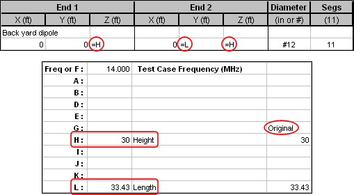
- Open a model file. If not done already, "variable-ize" those aspects of the model that you wish to have the optimizer automatically adjust. For example, with model BYDIPOLE.ez you could change both the
End 1 andEnd 2 Z coordinates from "30" to "=H" and theEnd 2 Y coordinate from "33.43" to "=L". Then on the Variables sheet assign values of "30" and "33.43" to variables H and L.Still on the Variables sheet, copy all the current variable values over to a spare column. (You can swipe through all the current values, press Ctrl-C, then Ctrl-V in a spare column.) As you are working with the optimizer you will most likely get confused and/or lost at some point. If you have the original values saved somewhere, like a spare column in the "scratch pad" area of the Variables sheet, you can just copy those values back to column C (the "Value" column) and be back to where you started. This is typically more convenient than re-opening the original model file. You can use other spare columns to save "interesting" or "has potential" sets of variable values as you experiment with the optimizer.
- On the Calculate sheet, run a single test calculation. Verify that the ground type, wire loss, plot type (azimuth or elevation), az/el angle, and plot step size are all as desired. On the Patterns sheet you may wish to take a snapshot of the "before optimization" pattern in order to give yourself a baseline for comparison.
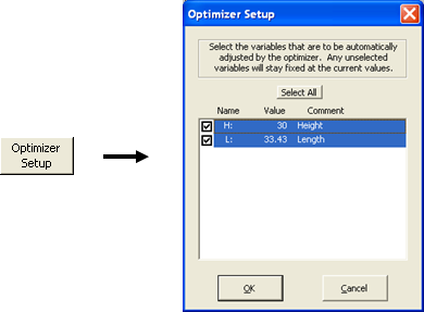
- Back on the Variables sheet, click the Optimizer Setup button. In the dialog window that follows select the variables that are to be adjusted and (if necessary) deselect others. Note that only those variables which have a "straight numeric" value setting are eligible for optimization. Any variables which are set via formulas referring to other variables cannot be optimized. For example, if variable A has a value of "10" it can be optimized, but if variable B is set via a formula such as "=A+5" it cannot be optimized.
If there are more than 10 "eligible" variable names use the up/down scroll bar in the dialog window to see all of them.
- When you click OK the "Optimize" sheet tab will appear.
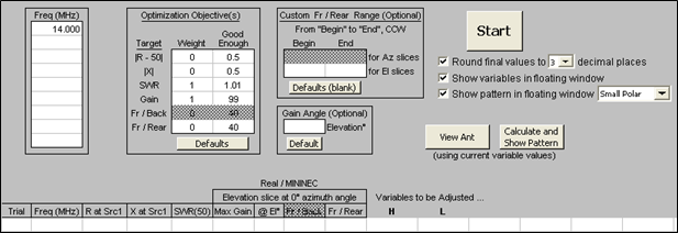
This is where you specify what the objectives are for the optimization process, as a combination of:
Frequencies:
You can optimize on up to 9 frequencies at the same time. This might be used to flatten the antenna characteristics across a band by specifying low, mid, and high frequencies for a band or portion of band. You can also use this feature to optimize a multi-band antenna.Targets:
- |R-50| - Best (lowest) absolute value of the quantity "source resistance minus 50". That is, get the source R as close to 50 as possible. For a target other than 50 use the small SWR Zo button on the Calculate sheet to choose a different (non-50) "Zo" value.
- |X| - Best (lowest) absolute value of the source reactance. That is, as close to resonance as possible.
- SWR - Best (lowest) SWR, using the current "SWR Zo" setting (typically 50).
- Gain - Best (highest) Gain. This is the max gain (total field) of the az/el plot type that is currently selected on the Calculate sheet.
- Fr/Back - Best (highest) F/B. AutoEZ defines F/B as the difference between the max gain of the az/el slice and the gain at the single point exactly 180° opposite the max gain point. (The max gain point need not be at 0° azimuth.) Note that F/B is not calculated for elevation plots over ground since in that case there is no field 180° opposite the max gain point.
- Fr/Rear - Best (highest) F/R. For azimuth plots and for elevation plots in free space, the standard AutoEZ F/R is defined as the difference between the max gain and the highest single gain found in the semi-circle opposite the max gain point. (Again, the max gain point need not be at 0° azimuth.) For elevation plots over ground, the standard AutoEZ F/R is defined as the difference between the max gain and the highest single gain found in the opposite quadrant. For use with the optimizer you can change those F/R definitions. See "Optional Custom Fr/Rear Ranges" below.
Weights:
To optimize on a single target set that target's weight to 1 and set all the other weights to 0 (or blank). To optimize on multiple targets at the same time set more than one weight to a non-zero value.Note: The weights are not percentages and they are not relative numbers. For example, if you set the SWR weight to 2 and the Gain weight to 1 it does not mean that you want a low SWR to be twice as important as a high gain. More details below.
Good Enoughs:
These are "don't give any importance to doing better than this" values. When/if the optimizer gets a particular target down to (or "up to" for Gain, F/B, F/R) the good enough value it will then try to improve on other targets (if any) that have not yet reached the good enough threshold.Good enough values are completely ignored if the corresponding weight is 0. Otherwise, they are used both for "single target" and "multiple target" optimizations. For single targets a good enough value will serve to shorten the optimization time since calculations will end when the good enough threshold is attained.
For multiple targets good enough values let you put realistic bounds on the targets. For example, suppose one solution yields a Gain of 10 dBi with an SWR of 1.2 while another solution gives Gain 10.2 dBi but with SWR 5.3. You probably wouldn't want to accept such a large increase in SWR for a mere 0.2 extra dBi in Gain. So you could assign "10" as a "good enough" Gain value. That way the optimizer will not treat "10.2" any different than "10" and will be free to search for solutions which have at least 10 dBi gain but with lower SWR values.
Optional Custom Fr/Rear Ranges:
These are used to let you minimize sidelobes in any direction, not restricted to just "rear" directions. For example, suppose a Yagi has max gain for an azimuth slice at 0° azimuth but also has major sidelobes roughly 45° off the main beam. Assuming the pattern is symmetric, you could minimize those sidelobes by setting the custom F/R range (for Az slices) to begin at 30° and end at 60° (thus incorporating the lobe at 45°), or to begin at 300° and end at 330° (thus incorporating the lobe at 315°). On the other hand you could begin at 30° and end at 330° if you wanted to minimize the lobes anywhere in that entire region, not just the forward-facing lobes.Allowing you to set both the begin and end of the range gives you complete control. No matter what direction the main lobe points, and no matter what sidelobes you want to minimize ("forward-facing" or "everything off the main lobe"), just look at the un-optimized pattern and pick the begin and end of the range you want to minimize. That is, the range in which the F/R ratio is to be maximized.
Note that the end value need not be greater than the begin value. For example, if the main lobe points at 90° and you want to minimize everything off the main lobe you could set begin to 120° and end to 60°. The custom range always starts at "Begin" then works counter-clockwise to "End".
As of maintenance release v2.0.15 you can specify up to four independent sets of F/R targets (eight sets as of v2.0.18, 24 sets as of v2.0.25), each with its own Weight, Good Enough, Begin, and End. Values for each set are separated by semicolons. You must specify the same number of sets (that is, use the same number of semicolons, if any) for Weight, Good Enough, Begin, and End. So, for example, if you want to use two custom F/R ranges you also have to use two weights and two good enoughs. You can include optional spaces around the semicolons to improve readability if desired.
If you use multiple custom ranges only the first one will show in the optimization log in the Fr/Rear column (column "I"). However, you can define the ranges in any order. If you defined the first range as 30 to 90 and the second range as 90 to 180, the
30-90 F/R dB value is what would show in the log. But if you are more interested in seeing the90-180 F/R as the trials progress you could define the first range as 90 to 180 and the second range as 30 to 90. Rearrange the weights and good enoughs to match.When using two ranges don't fall into the trap of thinking that the two fields are Begin1;End1 and Begin2;End2. You define them as Begin1;Begin2 and End1;End2 along with Weight1;Weight2 and GoodEnough1;GoodEnough2. If you want to use three ranges you'd use Begin1;Begin2;Begin3 and End1;End2;End3 along with three weights and three good enoughs.
A separate custom range (or set of ranges) applies to azimuth slices and elevation slices. Only one will be used for any given optimization run, depending on which plot/slice type is currently chosen on the Calculate sheet. The other (non-applicable) custom range(s) will be grayed out. When you specify a custom F/R range (or set of ranges) the begin and end values are shown in red if the set range (that is, "for Az slices" or "for El slices") matches the current Calculate sheet plot/slice type. The various target labels and log column headers are then also shown in red. This is just a visual reminder that a custom F/R range is in use.
Whether or not custom F/R ranges are used for optimization, the F/R value shown for normal calculations on the Calculate sheet will always use the "AutoEZ default" range.
Optional Gain Angle:
If you define the elements of your antenna to be parallel with the Y axis the main lobe will typically be at 0° azimuth. If you define the elements to be parallel with the X axis the main lobe will typically be at 90° azimuth. For arrays of vertical elements such as a 4 Square the main lobe may be at 45° azimuth. And of course for elevation plots over ground the main lobe may be at any elevation angle.For those reasons AutoEZ will always search for the maximum dBi value in the azimuth or elevation slice and define that as the "Max Gain" (or just "Gain") value. However, there may be situations in which you want to maximize the gain at a particular angle, such as when working with stack separations and you want to maximize the gain at a particular elevation angle. In that case you can set an explicit "Gain Angle" value and the optimizer will attempt to maximize the gain at that angle, not at just any angle in the slice.
When you set an explicit Gain Angle the value will be shown in red. The log column header will change from "Max Gain" to "Gain" and the header also will be shown in red. This is just a visual reminder that an explicit gain angle is in use.
See the "Tips and Tricks" section below for another example of using the Gain Angle field to prevent "swapping directions" of the main lobe.
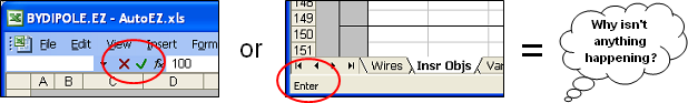
- Click the large Start button. If nothing happens when you click the button it's probably because you forgot to press Enter after making a target weight or good enough entry. In Excel, when you click on a cell and then type something (such as a number or a formula starting with an "=" sign), everything else is "frozen" until you complete the entry. You can do that by pressing Enter, by pressing one of the keyboard arrow keys, or by pressing the Tab key. But until you complete the entry, nothing else will happen.
If ever AutoEZ seems to be unresponsive, look up just to the left of the Excel formula bar near the top of the window. If you see a red X and green checkmark there, or if you look down in the lower-left corner of the Excel window at the Excel status bar and see "Enter" there, it means that Excel is waiting for you to complete the entry. In easy-to-remember graphical terms:
With that out of the way ...
For targets that are to be minimized, namely |R-50|, |X|, and SWR, AutoEZ will find a combination of variable values that results in a minimum target value. For targets that are to be maximized, namely Gain, F/B, and F/R, the negative of the target is used. That is, to maximize gain the algorithm will minimize the negative of the gain value.
When multiple targets are specified a "composite target value" is calculated as follows: First, each calculated result value is compared to the good enough threshold. If the value has attained the threshold it is clipped at the threshold limit. Then the (possibly clipped) value is multiplied by its corresponding weight. All such weighted values are added together. This process is repeated for each frequency and all the "per frequency" results are combined, always with equal weight to each frequency.
Here's an example for a single frequency. Suppose for a given trial solution the calculated SWR is 1.095 and the calculated slice Gain is 8.2 dBi. Further suppose the good enough SWR setting is 1.1 and the good enough Gain setting is 20. The SWR weight is 5 and the Gain weight is 2. The composite target value would be:
5 * (1.095 clipped at 1.1 = 1.1) + 2 * (-8.2 not clipped = -8.2)AutoEZ will then attempt to find other solutions which have a better (lower) composite target value. When the optimization process stops you can decide if you want to do another run with more or less weight assigned to SWR and Gain.
or
5 * (1.1) + 2 * (-8.2)
or
5.5 + (-16.4)
or
-10.9
- AutoEZ uses the Nelder-Mead simplex algorithm to converge on a target (or composite target) minimum. Unlike some other programs, AutoEZ does not calculate any derivatives or "steepest descent" directions.
Multiple sets of trial solutions are created with different variable values in each set. The number of sets is equal to the number of variables being changed plus one. Hence if you are optimizing on 2 variables AutoEZ will create 3 possible solutions, each having a different combination of variable values. The target value (or composite target value) is calculated for each set and the sets are ordered from best (lowest target) to worst (highest target). Remember, the goal is always to minimize the target, which for some targets (Gain, F/B, F/R) means minimizing the negative of the calculated value.
For each iteration the algorithm tries to move away from the set that produced the "Worst" (so far) target result. This has the effect of moving toward a better "Best" (so far) result. As the process continues both the best and worst results will get "better" (lower, minimized). The process stops when the worst and best sets produce equal results. That is, there is no longer a direction to move that will produce a better result.
Those trial solutions that produce a better "Best" (so far) target result are recorded in a log for later review if desired. In addition, you can watch the "Target Progress" fields that are shown just above the left side of the log. Note that many trial solutions will not improve on the "Best" (so far) target result. Those solutions are not logged. Although the algorithm must try such solutions to determine whether they are "better" or not, if they are not as good as a different solution already tried they are immediately discarded.
If you want to stop the process before the normal termination (that is, before the "Worst" so far solution target has caught up to the "Best" so far solution target) you can click the large Stop button. If EZNEC happens to be running a calculation (as indicated by "Waiting for EZNEC ..." in the status bar) at the moment you click the button the response will be delayed. It does no harm to click the Stop button multiple times. Once the click is recognized the button caption will change to "Wait", then the optimizer will (usually) run one more "final" set of calculations.
To save time, results that depend on the radiation pattern (Gain, F/B, and F/R) are not calculated if the weights for those three targets are all 0. The exception is that pattern data is always included for the first trial (the one that uses the start values for all variables) and the final trial (the one that uses the optimized, and possibly rounded, values for all variables). That way, even if you are optimizing on something like SWR only, you can see the pattern data in the summary rows that are shown at the end of the log.
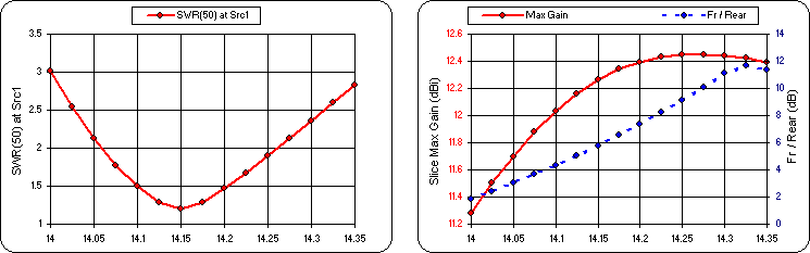
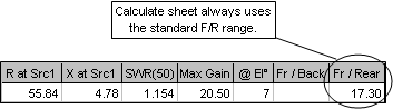
- As mentioned in the previous step you can watch the "Target Progress" fields along with the logged trials while the optimizer is running. Using the BYDIPOLE.ez example from above with default objectives (SWR weight 1, Gain weight 1, all other weights 0), below on the upper left is what you would see after 16 trials have been completed. At the start of the optimizer run (trial 1) the SWR was 2.292 and the Gain was 6.82 so the "Start" composite target value was
2.292+(-6.82) or-4.528. After 16 trials the "Best" so far trial (trial 16) SWR was 1.456 and the Gain was 8.60 so the composite target value was-7.144. At the same time the "Worst" so far (trial not shown) composite target value was-6.282 and the percentage difference between the two was 12.07%.As the optimizer continues the difference between Best and Worst will grow smaller. If you let the process run to completion the difference will be zero. At that point the Best so far set of variable values will be rounded, if you have elected to do so, to the number of decimals chosen. The Best-Worst percentage delta will be replaced with the Best-Final percentage delta. In this simple example the rounding still resulted in the same composite target value so the percentage delta is still zero. That is, the last Best so far trial (trial 34) used values for variables H and L of 42.644713 and 34.090425 respectively and the resulting composite target value was
-7.578. When those values were rounded to 42.645 and 34.09 it made no difference in the Final composite target value, still-7.578. When the optimizer stops, either by normal completion or because you clicked the Stop button, the Start and Final log entries are shown together (below, bottom) so you can easily judge the quality of this run and decide if you want to do another run, perhaps using different target weights.
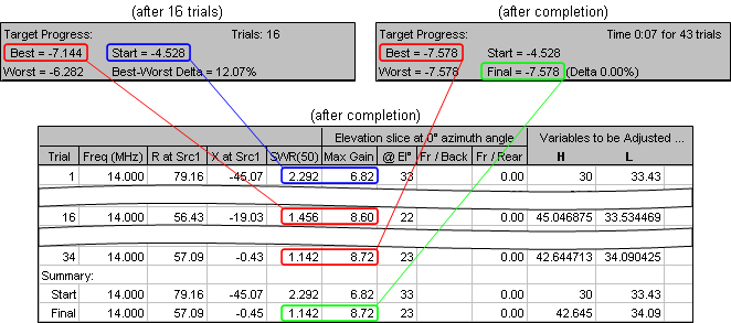
Notice that the "Start" row is just a copy of the trial #1 row and the "Final" row is almost the same as the last "Best so far" row (trial #34 in this example) except the variable values have been rounded and the results recalculated. Look closely and you'll see that the rounding changed the "X at Src1" result from
-0.43 to-0.45 although that produced no change in the SWR, at least with the precision shown.
"Local" Best Solution vs "Global" Best Solution
Like many optimizers, AutoEZ finds a "local" best solution. That is, if you let the process run to completion you can be sure that there are no better combinations of variable values "nearby". However, that doesn't mean that you have found the absolutely best solution. You may or may not be able to find a slightly better solution by re-starting the process after it has completed once (which will automatically begin with a slightly different set of start values) and/or by manually creating a different set of start values.
For example, suppose you were optimizing the BYDIPOLE model only on Gain and you were changing only the Height. Here's what the plot of "-Gain" (negative gain, which is to be minimized) vs Height looks like.
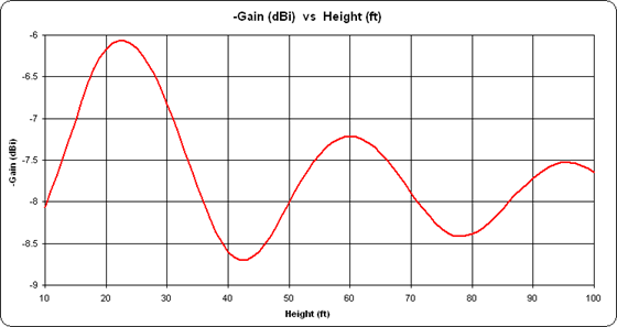
As you can see, if the initial value for Height was somewhere in the range of 30 to 50 ft the optimized Gain (minimum -Gain) would be found near 42 ft. But if the initial value for Height was in the range 70 to 90 ft the optimized Gain would be found near 78 ft.
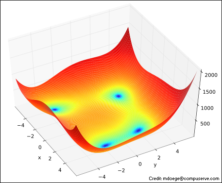
This same concept can also be illustrated by using an example from the realm of numerical analysis and optimization theory, not directly related to antenna modeling. Many different "standard test cases" have been developed to determine the efficiency of a given optimization algorithm. One such test is Himmelblau's function, a function of two variables (x and y) defined as:
f(x, y) = (x2 + y - 11)2 + (x + y2 - 7)2This function has four identical local minima:f(+3.000, +2.000) = 0.0When plotted in 3D with both x and y in the range ±6 it looks like this, with the minima in the centers of the dark blue regions.
f(-2.805, +3.131) = 0.0
f(-3.779, -3.283) = 0.0
f(+3.584, -1.848) = 0.0
Below is a contour (top-down) view of the same function showing how the Nelder-Mead algorithm would converge on one of the minima. Since there are two variables (now shown as x1 and x2) the algorithm computes function values at three points. Those three points are shown as the corners of the red triangle. The triangle "walks" (or "flops" if you prefer) away from the worst of the three points for any given iteration, changing shape as it goes, and eventually converges to one of the Himmelblau minima. The small "preview frames" shown first let you see where the triangle starts and where it ends. The large animation plays continuously.
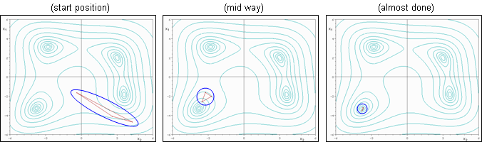
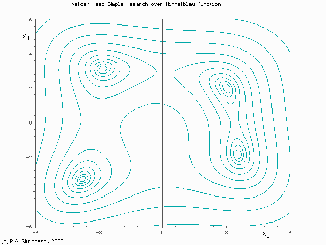
(Press Esc to stop the animation, F5 to restart.)As you can imagine, if the initial triangle had been placed at a different start position it would have converged to a different minimum. And keep in mind that this is a very simple example using a well-defined function of only two variables. With three variables, the algorithm could be visualized as a
4-sided tetrahedron flopping its way through 3D space rather than a3-sided triangle in 2D space.With even more variables the process is hard to visualize but still works mathematically. For example, with 31 variables the "triangle" would be more like a
32-sided soccer ball polyhedron, always rolling away from the worst point in31-dimensional space, where each colored area on the ball's surface represents a different combination of variable values and the ball is squashed into different shapes as it rolls in different directions.
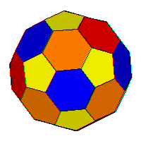
That should make your head spin, especially trying to picture
31-dimensional space.
Optimizer Tips and Tricks
Here are some other tips and tricks for using the optimizer.
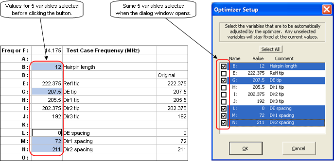
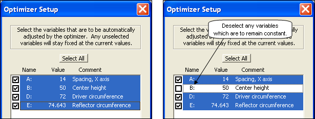
- On the Variables sheet, before clicking the Optimizer Setup button you can pre-select multiple variables by selecting any cell in that variable's row. You can drag through to select multiple variables (multiple rows) and you can use the Ctrl key to select discontiguous sets of variables. Then when you click the Optimizer Setup button any eligible variable names in the selected rows will be "pre-selected" in the dialog window. You can then add more, drop some, or make any other changes. This is easier than always having to select one at a time in the dialog window. You can also click the Select All button in the dialog window and then, if necessary, deselect some variables.
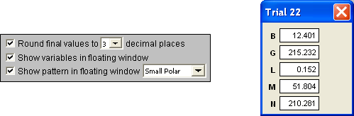
- There are three optional check boxes just below the large Start button. The first, already mentioned above, allows you to round the final values to a specified number of decimals. In order to converge to a solution the optimizer must work with very precise values. However, there is no way you could measure and cut an element to be (for example) 1.23456789 meters in length. This first option lets you see what the final results will be with all values rounded to (for example) the closest millimeter. If you choose rounding, when the optimizer stops (either normal completion or early termination if you don't want to wait for the last little bit of improvement) you can see if the rounding made any difference by looking at the "Target Progress" numbers. If "Final=" is not the same as "Best=" then the rounding made a difference, since the "Final" set of calculations is done with rounded values.
The second check box lets you see all the variable values in a floating window as the optimizer is running. In the floating window the values are always displayed with whatever you have chosen for the rounding number of decimals, if any. That makes it possible to visually track changes as the optimizer is running, which would be hard or impossible to do if all the decimal points in the floating window did not line up. If the trial number in the title bar changes but the values themselves don't seem to be changing it's because the changes are below the level of the displayed precision.
The third check box lets you see the radiation pattern for every logged trial. You can choose to see either a polar or rectangular pattern, in one of three sizes. If you are optimizing on multiple frequencies the floating pattern window can show any of them but only one at a time. Use the dropdown in the floating window to pick a different frequency to view. (Action will be a little jerky since EZNEC is hogging most of the CPU.) If you want to start out with a particular frequency, put the Excel selection box on the frequency of interest (cells B2-B10) before clicking Start. If the Excel selection box is somewhere other than a frequency when the optimizer starts, the first frequency is chosen by default.
Note that the third check box is disabled if the Gain, F/B, and F/R weights are all zero. Except for the first and final trials no pattern data is collected in that case so the optimizer can run faster.
Only those trials which are logged, that is, which improve the "Best so far" target value will be used to update the two floating windows. The windows will stay fixed until a new "Best so far" trial is encountered. The floating variables window takes virtually no extra time to show. Use of the floating pattern window may cause a noticeable delay with versions of Excel prior to 2003.
Both floating windows can be repositioned as you like. The positions will be remembered. However, the windows can be repositioned only after EZNEC has returned control back to AutoEZ for any given trial. A trick is to click and hold on the window title bar until the optimizer pauses, then move the window. When you release the mouse button the optimizer will continue. This same trick may be used if you see an "interesting" pattern as the optimizer is running. Assuming you are quick enough with the mouse you could click and hold on the title bar, giving you time to study the pattern in more detail and possibly note the trial number for later use. See the discussion of the Reset buttons further below.
You can close the floating window(s) while the optimizer is running but you can't show them again until the next start. If a window is open already there is no need to close it before the next start. Both floating windows are closed automatically whenever you tab to a different sheet.
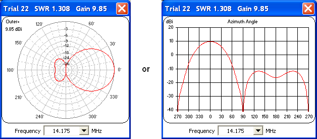
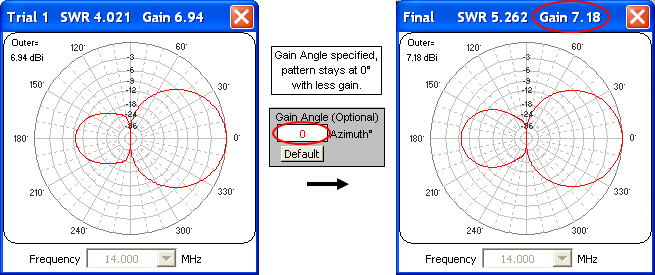
- When working with certain types of parasitic elements and maximizing Gain you may find that the pattern "swaps directions" unexpectedly. That's because unless you specify otherwise the optimizer will attempt to maximize gain at any angle in the azimuth or elevation slice. For example, the illustration below shows the pattern at the start (Trial 1) and end (Final) of a run. The gain value has increased from 6.94 dBi to 7.38 dBi but the pattern points in the "wrong" direction.
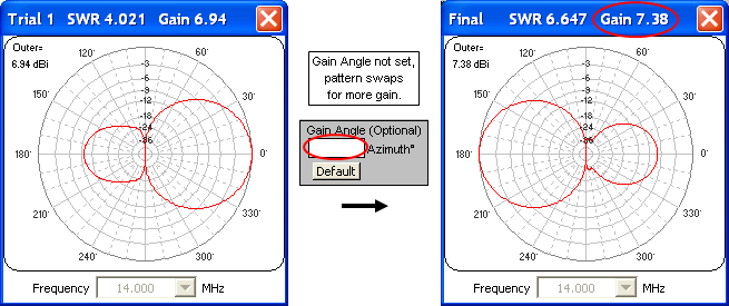
You can prevent that by setting the Gain Angle (cell H9) to a desired value such as "0". The optimizer will then maximize gain only at the specified angle.
In this example, where the Gain Angle has been set to 0, the gain does not increase by as much but the pattern stays pointed at 0° azimuth.
- When learning to use the AutoEZ optimizer one of the first questions that many people ask is "How do I limit the range of a variable?" There is an easy way to do that but you are encouraged to use this technique only as a last resort. In other words, first try to understand the results of the optimizer without any restrictions on the variables. You may be surprised at what you find.
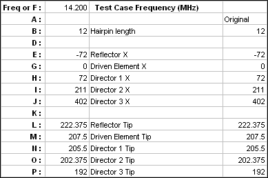
For example, with a 4 element Yagi (Reflector, Driven Element, Director 1, Director 2) and given a particular set of objectives that you deem suitable, you may find that the boom "wants" to be 288 inches (24 ft) long. You'd like to limit the boom to 240 inches (20 ft). Before you do that, take some time to study the situation. If the Reflector has X coordinates of 0 you could manually set the Director 2 X coordinates to 240 and then just not include that variable in the optimization. Take a look at both the resulting pattern and the current distribution on the four elements. You may find that you can achieve the same objectives with just three elements, not four. You would never have discovered that if you just arbitrarily decided that you wanted four elements on a 240 inch boom.
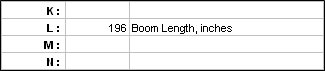
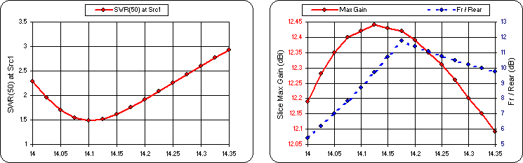
If you still want to limit the boom length to "no more than 240 inches" as opposed to "exactly 240 inches" here's how. Suppose the X coordinate for the final element, whether that is Director 1 or Director 2, is controlled by variable L. If the initial value for L is 196 the entry on the Variables sheet might look like this.
Rather than using a straight numeric value for L and having the optimizer adjust that value you can enter a simple formula for L and have the optimizer adjust a related straight numeric value. For example, you might set up something like this.
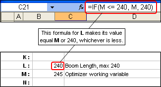
The optimizer will adjust variable M. Variable L, which still controls the wires of your model, will use the value for M but only if that value is <= 240 inches (20 ft). If the optimizer sets M to more than 240, perhaps to 245, L will stay at 240.
If the variable in question is referenced only once in your model it may be more convenient to just modify the formula where the variable is used rather than creating a second, proxy variable. For example, suppose you have an R±jX type load using variable B for the resistance and you want to insure that the value is always non-negative. You could use a formula like this.
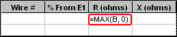
Use of "=MAX(...)", or possibly "=MIN(...)", is an alternate way do the same thing as the use of
"=IF(...)". And note that in regions were the decimal separator is a comma, the arguments of Excel functions are separated by semicolons.
Here's another trick involving use of proxy variables, especially applicable when modeling Yagis. It's unlikely that you can actually build to a tolerance any better than 1/16 inch (or maybe even 1/8 inch). So there's no point in letting the optimizer quibble over a dimension of, say, 170.92" vs 170.93" when you can't build to 0.01" anyway. Note that the "Round final values to x decimal places" option only applies to the final calculation, not to intermediate trial calculations.
To force each optimizer trial to use rounded values you can use "pass-through" (proxy) variables. And to force rounding to the nearest 1/16" as opposed to a number of decimal places you can use the Excel MROUND function. (MROUND is "round to the nearest multiple of".) Here's how that would work.
Let's say you are using variable A to control some aspect of the model. Define a new variable, say AA, for use by the optimizer. Give AA the same value that is currently set for A. Then use this formula for original variable A:
=MROUND(AA, 1/16)
Do the above for all variables that control element tips and boom positions. Now optimize on AA, not A, along with the other "for the optimizer" proxy variables that you have defined. That way, if the optimizer changes AA from 170.92 to 170.93 the actual value for A as used on the Wires sheet will not change. It will stay at 170.9375 which is 170+15/16. And since the model itself has not changed there will be no difference in the calculated results, hence the optimizer won't waste any more time trying to change that variable with smaller and smaller step sizes.
You'll find that the optimizer will run to completion much faster and all the final values for the "original" variables (like A) will be rounded to the nearest 1/16" even though you might see a different value for the "optimized" variables (like AA).
With Excel 2003 or earlier you must enable the "Analysis ToolPak" add-in to use MROUND. (Click on Tools > Add-Ins and make sure "Analysis ToolPak" is checked, not to be confused with "Analysis ToolPak - VBA" which is not needed.) With Excel 2007 and newer no special action is needed.
When working with length units of Meters or Millimeters you can use the same "proxy variable" idea but you need not use the special MROUND Excel function. If you want to round to the closest millimeter when length units are meters, just use
"=ROUND(AA, 3)". If length units are already millimeters, use"=ROUND(AA, 0)" to round to the closest integer millimeter.
- When you request an elevation plot over ground the F/B ratio is not calculated since in that case there is no radiation exactly 180° opposite the main lobe. To avoid any confusion the F/B weight and good enough target fields and the F/B column header in the log will be grayed out. This is just a visual reminder that F/B is not used for elevation plots over ground.
- AutoEZ is frozen while the EZNEC "Running NEC" window is visible, which is also when the Excel status bar shows "Waiting for EZNEC ...". Although completely optional, you might want to arrange your desktop to make it more obvious what's happening. You could resize the Excel (AutoEZ) window so it does not occupy the entire screen. Then move the main EZNEC window off to the upper right so at least a portion of it is visible. Finally, move the EZNEC "Running NEC" sub-window to the lower right so it also is visible.
Normally the EZNEC "Running NEC" sub-window is in the center of the screen, underneath the Excel window. To move it, it has to stay open long enough for you to grab the title bar. Using EZNEC (not AutoEZ), open any large model and request a 3D plot with 1 degree step size. Then when you click the EZNEC "FF Plot" button the "Running NEC" window should stay open for more than an instant. Grab it and move it. Once moved you can click the "Cancel" button.
Here is a much-reduced screen grab to illustrate.
- The View Ant and Calculate and Show Pattern buttons will always use the current variable values as shown in column C on the Variables sheet. That might be the values before the optimizer is started, after the optimizer completes normally, after it is manually stopped, or after you use either of the Reset buttons explained in the next bullet.
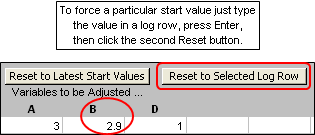
- There are two Reset buttons, neither of which will show until you have run the optimizer at least once. The one on the left (Reset to Latest Start Values) allows you to "do over" starting from perhaps a known good design but using a different set of target weights. The one on the right (Reset to Selected Log Row) allows you to set the variable values to what is shown in any log row. Just select anywhere in the desired log row (a row with variable values) before clicking the button.

The second button may be useful if you notice an "interesting" trial result during optimization. You can easily set the variable values to that trial and then click the Calculate and Show Pattern button to investigate further. If you want to then revert to the "Final" values just select that log row and click the button again.
- The optimizer setup fields are stored in .weq model files. When you open a .weq file that has that data included: a) the Optimize sheet will be made visible automatically, b) all the header fields will be set as they were when the model was saved, and c) the optimized variables will be shown. So if you open a model file you'll be right back to where you were and if you send a file to somebody else there will be no confusion as to what targets were used.
If you open an .ez file or an older .weq file the Optimize sheet header fields will be set to default values and the sheet tab will not be visible until you click the Optimizer Setup button on the Variables sheet.
- You can switch to other windows (web browser, email, whatever) while the optimizer is running.
- And the most important tip of all: When working with anything other than the simplest of antennas, don't fall into the trap of thinking you can set up a complex set of optimizer objectives, click Start, walk away for a few hours, and come back to find a perfect design. You'll get much better results if you think of optimization as a process of stepwise refinement rather than a one-shot deal. The next example will illustrate this.
Loop Sizes and Spacing with 'Sample Quad B.weq'
Suppose you wanted to optimize a 20M quad. You want to use it over the entire band and you want a direct
50-ohm feed.Open model file 'Sample Quad B.weq'. This is a variant of the model discussed in detail in the Modeling with Variables - Manual Entry section. The dimensions are based on various rules of thumb given in The ARRL Antenna Book.
On the Calculate sheet, click the Generate Test Cases button and set up a frequency sweep for the 20M band.
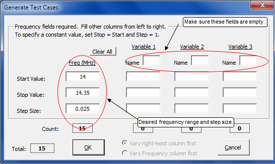
Calculate and tab to the Triple sheet.
Obviously this does not meet your criteria so let's put the optimizer to work. Tab to the Variables sheet. The first thing to do is make a copy of all the current variable values so you'll have a record of where you started. Swipe through all the current variable values (cells
C12-C15), press Ctrl-C, select cell E12, press Ctrl-V. Without changing the new range of selected cells, click the Optimizer Setup button. That is, these are the selected cells when you click the button.
Let's assume that you want to keep the boom at 50 ft. Just deselect that variable before clicking OK. If you are optimizing on more than just a few variables this is a convenient way to select the ones to be changed, rather than selecting each one individually. In this case you could have also just clicked the Select All button and then deselected variable B.
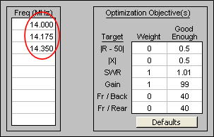
On the Optimize sheet enter bottom, mid, and top frequencies for the 20M band. For now, leave all the other setup fields with the default settings.
Click Start. For this particular scenario the optimization won't take very long but you are always free to open other windows to do things such as check your email while the optimizer is running.
When the run finishes you can see the numeric results in the log. To see plotted results you could click the Calculate and Show Pattern button and then tab to the other sheets to see different plots, but the calculations would be for only the three frequencies used during the optimization. So instead, tab to the Calculate sheet and click the Generate Test Cases button again. You will find that your frequency sweep setup entries have been preserved, so just click OK, do a calculate, then tab to the Triple sheet.
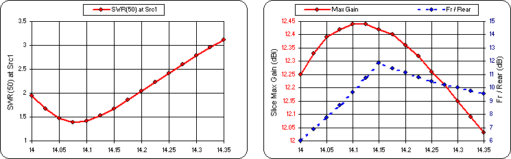
That's better but there is still room for improvement. The minimum SWR and the maximum gain do not fall in the middle of the band. Also, let's see if it's possible to lower the minimum SWR (as well as shift it) without giving up too much gain.
Tab back to the Optimize sheet and change the setup as follows.
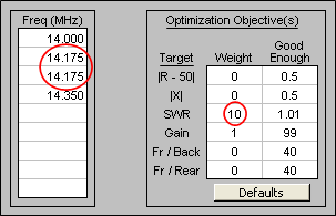
The SWR weight has been increased from 1 to 10. That means that more importance will be given to a low SWR, possibly with a trade-off of less gain. For shifting the frequency response, although there is no method to give "weights" to the various frequencies, you can do the same thing by duplicating one or more frequencies. In this case 14.175 is entered twice, so the results at that frequency will have twice the weight as the results at other frequencies.
Run the optimizer again, starting with the variable values as set at the end of the previous run. (That is, do not reset the values.) Then tab to the Calculate sheet, set up a frequency sweep again, calculate, and tab to the Triple sheet.
The SWR curve is a little better but it cost you about 1 dB of gain at the low end. And the Fr/Rear ratio at 14 MHz is only 2 dB, not very good at all. Let's keep trying. Back to the Optimize sheet and give the Fr/Rear target a non-zero weight.
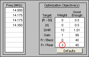
Which gives this.
Not bad. Feel free to keep experimenting.
Element Lengths - Element Spacing - Hairpin Match with 20M5ELYA.ez
The next example will use a model that has not yet been "variable-ized". It will also demonstrate a technique to build a Yagi model from scratch, complete with "stepped diameter" wires for each element.
Open model '20M5ELYA.ez' which is one of the standard EZNEC samples. This is a 5 element Yagi for 20 meters with a total boom length from reflector to third director of 474 inches, not quite 40 ft. (It's 40 ft when you include an extra 3 inches at each end for mounting plates.) The elements are constructed from telescoping aluminum tubing with a fairly complex taper schedule, six different diameters duplicated on each side of the boom.
The design has already been optimized for (azimuth) F/R > 20 dB and SWR < 2:1 over the entire 20M band; however, that SWR bandwidth assumes that a perfect 1:1 match is achieved at some particular frequency via a hairpin matching network which is not included in the original model. We'll modify the model to demonstrate how to add a hairpin.
On the Calculate sheet, set up a frequency sweep for the 20M band using the Generate Test Cases button, make sure the plot type is azimuth at 0° elevation angle, and do a calculation. Here's what you'll see if using the EZNEC
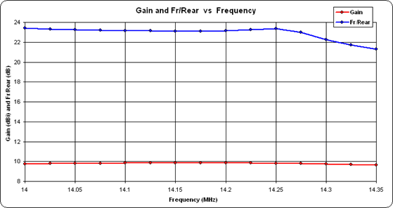
NEC-2D engine and EZNEC's stepped-diameter correction. Results will differ slightly if using theNEC-4D engine.
Note that the minimum SWR value is 2.4, not 1.0. Also, don't be misled by the shape of the gain curve. The range of the left-hand (red) Y axis scale is only 0.19 dB. Over the entire 20M band the gain varies from 9.84 to 9.65 dBi, constant for all practical purposes. If you prefer you can tab to the Custom sheet, plot "Slice Fr/Rear" vs "Frequency", take a snapshot, then plot "Slice Max Gain". That makes it more obvious that both parameters remain fairly flat across the entire band.
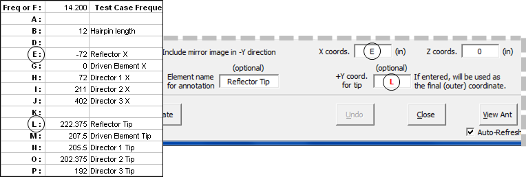
The first order of business is to assign variables. It is not necessary to do this for every coordinate value. The taper schedule for the interior portion of each element will remain fixed so only the tips need to be adjustable.
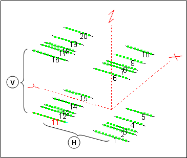
Here's a top-down view of the wires.
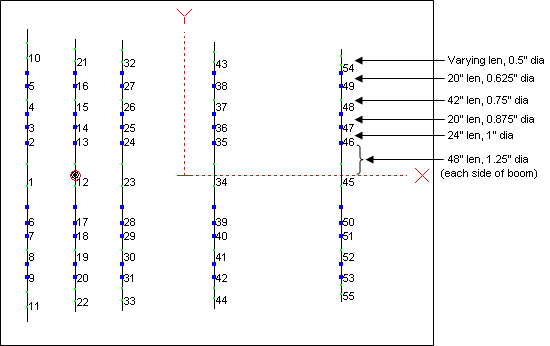
The positive
End 2 Y coordinates for wires 10, 21, 32, 43, and 54 are the tips. (The negative coordinates are identical except for the sign.) The X coordinates for those same five wires will be used for illustration, although in most cases you would put the Reflector on the Y axis (X = 0) and just use variables for the other four elements. This is a Free Space model so all the Z coordinates will be left at 0.Do the five X coordinates first. Copy those values from the Wires sheet to the Variables sheet and add some annotation. Remember, it is not necessary to do the Copy/Paste one cell at a time. On the Wires sheet you can select cell E20 (for example), press and hold the Ctrl key, then select E31, E42, E53, and E64. With those five cells all selected press Ctrl-C. Then tab to the Variables sheet, select a desired empty cell in the C column, and press Ctrl-V. In the D (Comment) column add some brief annotation so you can keep track of which variable does what.
Repeat this process for Wires sheet cells F20, F31, F42, F53, and F64. Be sure to select the positive Y coordinate, not the negative value which is in the next cell down.
Since we'll be adding the hairpin in just a moment, pick a spare variable for the hairpin length and give it a nominal initial value such as 12 inches. Finally, copy all the values to a spare column so you'll have a record of where you started.
When you're done the Variables sheet might look like this.
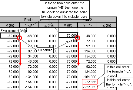
Next, replace the appropriate coordinate numerical values with formulas that use the associated variable name. There are a variety of ways to do that. The simplest is to just select a cell, type the appropriate formula, and press Enter. If the same formula is to be used in a group of cells, such as for the X coordinates that all have the same value, you can take advantage of the Excel fill handle. For example, here is what you would do for the wires that make up the Reflector, where the objective is to replace all the X coordinate values of
"-72" with the formula "=E" and replace just the twoEnd 2 ±Y coordinate values of "222.375" and"-222.375" with "=L" and"=-L" .
Repeat for the other four elements. It takes much longer to describe than to do.
A second method is to use the AutoEZ Replace XYZ Numbers with Formulas feature. With that you select a number to be replaced and enter the appropriate formula in a dialog window. AutoEZ will scan all the X,Y,Z coordinates searching for the number or its equivalent negative value. For each such number found, the formula or the negative equivalent of the formula will be automatically entered as a replacement.
A third method is to just rebuild all the wires of the model. Believe it or not you've already done most of the work in picking variable names and setting initial values. The technique will be explained here as a way to replace an existing model, but keep in mind you could do the same thing when building a new model.
On either the Wires or Variables sheet click the Stepped Dia button. If you are just trying to build a model from published specifications such as in a book or magazine, without worrying about variables, you may find it more convenient to work from the Wires sheet. For this example, since you want to use variables in your model and you already have the variable names and initial values set, it is more convenient to do most of the work from the Variables sheet.
When you click the Stepped Dia button a dialog window titled "Create Set of Stepped Diameter Wires" will appear. The very first time you use the dialog all the fields will be empty; after that, the fields will retain the last-used values.
Assuming you have not already set any values, the first thing to do is enter the "taper schedule" for the inner sections of the elements. The information you need can be found on the Wires sheet. You can switch back and forth between the Wires and Variables sheets without closing the dialog window.
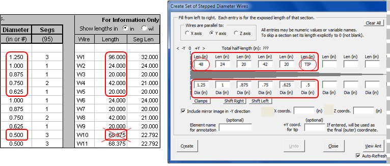
Notice that two of the length entries are not what you might be expecting. On the Wires sheet the length of the first wire in the set is shown as "96" inches. But notice that there is only one entry for "1.250" diameter. That's because the first wire of each set spans from
-Y to +Y across the boom. In the dialog window you always enter section lengths for just the positive half of each element. Hence "96" becomes "48" in the taper schedule.The second unusual length entry is for the final ".5" inch diameter section. You need to enter something in that length field; you can't leave it empty and you can't enter an explicit "0". But you don't really have to enter the actual length of the tip section since that will change for each element. You could enter "999" if you like, or "N/A", but "TIP" works well also. Anything other than empty or "0" will do. (As of maintenance release v2.0.25, if a tip coordinate override is present it is no longer necessary to enter a dummy value for the final section length. You can leave the final length empty.)
Now, without closing the dialog, take a deep breath and click the small Clear All button on the Wires sheet (not the Clear All button in the dialog window). In cell B10 on the Wires sheet enter a new title for your model, perhaps something like "Rebuilt 5 el Yagi".
The rest is easy. Again, without closing the dialog window, tab back to the Variables sheet so you can refer to the variable names. Then use the dialog to build five elements, one at a time, starting with the Reflector. Enter "E" in the "X coords." field, enter "0" (zero) in the "Z coords." field, and enter "L" in the "+Y coord. for tip" field. Notice that when you make that last entry the "Element name for annotation" field is automatically set to whatever comment is associated with variable L. You are free to modify that if you wish, such as removing the "Tip" letters. Click Create. All of the wires that make up the Reflector will be added to the Wires sheet.
You can tab back to the Wires sheet to see what got created but it is probably more convenient to stay on the Variables sheet. That way you don't have to try to remember what variable does what.
The dialog window will stay up after you click Create. Replace "E" with "G", replace "L" with "M", and click Create again to create the Driven element wires. Repeat for the three Directors. After the last element is created you can click Close.
You're done creating all the wires for the replacement model. On the Wires sheet you can change the annotation for each set of wires if you wish. The blank row between each set makes it easy to distinguish one from another. Also notice that, unlike in the original model, the wires for each element have been created in order from the "most negative" to "most positive" Y coordinate. That has certain advantages when viewing the chart on the Currents sheet tab as explained in the Cautions for the Currents Chart section.
Important: Because the new wires have been created in a different order the source placement on the Insr Objs sheet is now incorrect. Change the source placement from wire 12 (original model) to wire 17 (replacement model). Then use the View Ant button to verify that everything is as it should be.
Now for the hairpin match. A hairpin is nothing more than a small length of parallel conductor transmission line, shorted at one end to make it a stub and with the other end connected to the feedpoint. It will cancel out any feedpoint reactance and in the process transform the feedpoint resistance to 50 ohms.
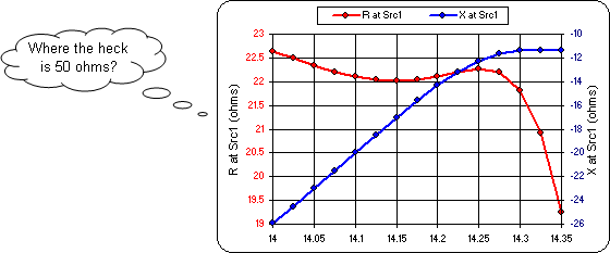
Tab to the Triple sheet and look at the R/X plot. You may be wondering how you are going to get 50 ohms out of any of that.
The trick is to remember that the hairpin (shorted transmission line stub) will be connected in parallel with the feedpoint, so you need to know the parallel equivalent of the series form R and X values. Here are the formulas along with a diagram from The ARRL Antenna Book.
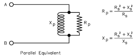
You can see that if the Xp component were to be removed, or in this case canceled by connecting another Xp component (the hairpin) in parallel with the same magnitude but opposite sign, the only thing left would be Rp. So what are the equivalent Rp and Xp values?
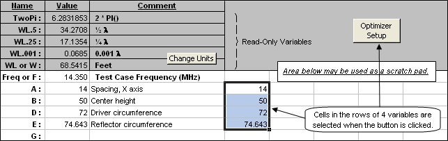
As explained in the User-Defined Result Columns section, you can let Excel do the calculations for you. On the Calculate sheet, enter an unused variable name, say U, in cell C10. In cell C11 enter the formula
=(G11^2 + H11^2)/G11
which will calculate the parallel form resistance, Rp. Use the fill handle to duplicate the formula down to the last frequency row. Enter another unused variable name, say V, in cell D10. In cell D11 enter the formula
=(G11^2 + H11^2)/H11
and then fill down to calculate the parallel form reactance, Xp. Here are the results.

An Rp value of exactly 50 would fall somewhere between 14 and 14.025 MHz. It could be shifted to a different place in the band by adjusting the driven element tip lengths. The corresponding Xp value is roughly
-46 ohms. If that reactance is canceled with +46 ohms provided by the hairpin (connected in parallel), the only thing left would be a pure Rp of 50 ohms. And when there is zero reactance, the parallel form resistance is exactly the same as the series form resistance. Presto.To add the hairpin to the model tab to the Insr Objs sheet. In the first row of the Transmission Lines table enter "17" and "50" for the
End 1 connection, the same as where the source is placed. (That's assuming you followed the above steps to rebuild the model. If not, the source is on wire 12, not 17.) When a transmission line and source are placed on the same segment EZNEC connects them in parallel. Enter "Short" (or just "S") for theEnd 2 connection. For the Length enter the formula "=B", recalling that earlier we gave B a nominal value of 12 inches just as a starting point.Now what about the remaining fields? You could manually enter appropriate values but there is an easier way. Click the Set Zo, VF, and Loss button. In the dialog window select the "Parallel Conductors" option and then enter appropriate values for wire diameter, wire spacing, and frequency. The "#12" and "3" are typical values but you could enter whatever is used for your actual hairpin.
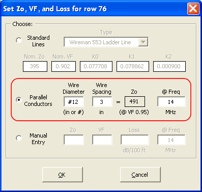
AutoEZ will compute both Zo (given an assumed velocity factor for open wire line) and the loss in
dB/100 ft at the frequency you specified. EZNEC will adjust that loss for other frequencies as necessary.When you click OK here's what the complete transmission line definition would look like.

Now what we need to do is adjust the driven element tip lengths to move the Rp=50 point to a chosen frequency and then adjust the length of the hairpin to cancel out the Xp value. Sounds to me like a job for the optimizer.
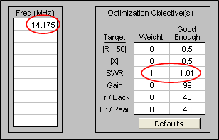
Tab to the Variables sheet and click the Optimizer Setup button. Select only variables B and M to be adjusted. For now, leave all the other variables at their current values. On the Optimize sheet enter a single frequency of 14.175. Set the SWR weight to 1 and set all the other weights to 0. You can leave the SWR good enough at 1.01 which for all practical purposes is a perfect match.
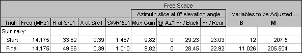
Click Start. For each trial EZNEC will compute the impedance at
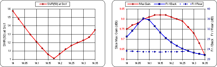
End 1 of the hairpin using the equivalent of the full transmission line equation, not just an approximation for ideal line. That impedance will be combined in parallel with the source impedance at the center of wire 17 as computed by the NEC engine. The result will be passed back to AutoEZ. The AutoEZ optimizer will "flop the triangle" around, using different values for variables B and M, until the SWR value meets (or passes) the good enough threshold. In less time than it took to read this paragraph you'll have the B and M values needed for a perfect (almost) match.
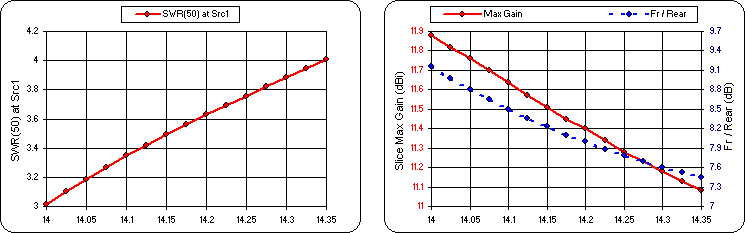
Tab to the Calculate sheet, use the Generate Test Cases button to set up a frequency sweep, then calculate.
Not bad. The design criteria of SWR < 2:1 over the entire band is met and the Gain and F/R response curves are essentially unchanged. Now let's turn the optimizer loose to adjust more than just the hairpin and driven element lengths, while shooting for the best SWR, Gain, and F/R over the entire band. It'll be interesting to see what compromises need to be made.
Although it would be possible to adjust all the variables, for this example let's assume that the boom length stays fixed at 474 inches (from
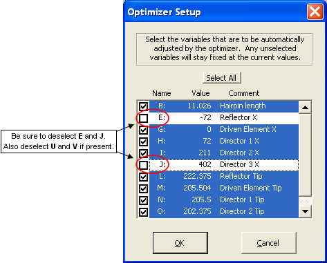
-72 to +402 on the X axis). On the Variables sheet click the Optimizer Setup button, click Select All, but then deselect variables E and J. That means that the hairpin length can change, the X axis spacing for the middle three elements can change, the lengths for all elements can change, but the overall boom length will stay fixed. If present, also deselect variables U and V. They were used merely for illustration and play no part in the model itself.
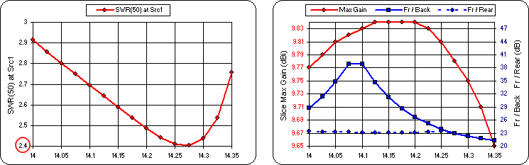
On the Optimize sheet enter frequencies of 14, 14.175, and 14.350. Set the weights for SWR, Gain, and F/R all to 1 and leave the corresponding good enough values at the "go for broke" thresholds. Go.
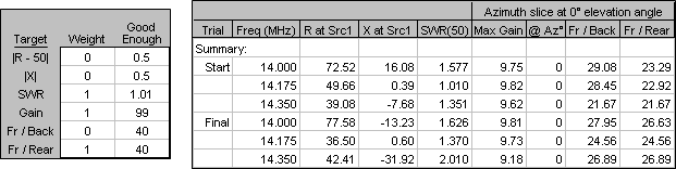
Not so good and here's why. The final F/R value is roughly 26, the Gain value is roughly 9, and the SWR value is roughly 2. Since these numbers are not close to being equal, by giving a weight of 1 to each of these three targets the calculated composite target value is dominated by the F/R number. In effect you specified that F/R was "more valuable" than the other two targets and that's exactly what you got. F/R improved substantially, Gain was a wash, and SWR got worse.
Let's try again. Click the Reset to Latest Start Values button. Set the SWR weight to 20 with a good enough threshold of 1.2. Set the Gain weight to 5. Leave the F/R weight at 1 but set the threshold at 20 which was the original design criteria. Basically you are trying to eke out a bit more gain while keeping acceptable SWR and F/R numbers across the band.
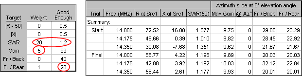
That's better. The SWR response actually improved although that wasn't really a goal, the F/R response continued to meet the criteria of > 20 dB across the band, and you did indeed get slightly more peak gain.
Here are some ideas for other experiments.
- See if you can get a direct
50-ohm feed without using a hairpin match by adjusting the driven element tips and the three spacings. If you like you can just temporarily "mark out" the hairpin by entering an "x" in cell A76 on the Insr Objs sheet, rather than deleting the entire row.
- Work with a more "real world" scenario. On the Wires sheet use the Move/Copy button to raise all the wires by some nominal amount such as 600 inches (50 ft). On the Calculate sheet, change the ground type from Free Space to Real and change the wire loss from Zero to Aluminum. Use the optimizer to see how the dimensions might change while still meeting the original design criteria.
Separation in a 2x2 Stack with 'W5TX 2M5WB375 Stack With Feed.weq'
This example will demonstrate how a custom F/R range might be used. Open model file 'W5TX 2M5WB375 Stack With Feed.weq'. This model was used in the 2 Meter Yagi, Stack and Feed section to demonstrate how to feed a 2x2 stack. In this example we won't change the feed system or any dimensions of the four Yagis in the stack. Instead we'll experiment with adjusting the horizontal and vertical separation of the individual antennas by adjusting variables H and V.
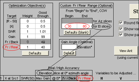
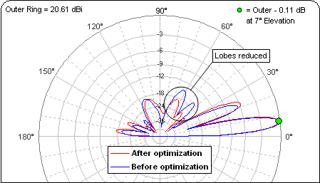
As always when using the optimizer you'll want to tab to the Variables sheet and copy the existing values to a spare column. Then on the Calculate sheet change the plot type to elevation at 0° azimuth angle, calculate, and tab to the Patterns sheet. Take a snapshot of the elevation pattern to serve as a "before optimization" reference. Back on the Variables sheet click the Optimizer Setup button and then Select All to select both H (Horizontal separation) and V (Vertical separation) to be adjusted.
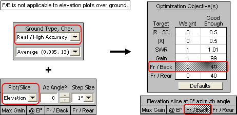
For this example suppose your objective is to minimize the forward-facing high-angle lobes of the pattern by adjusting the stack separation variables. As mentioned earlier in the overview, for elevation plots over any type of ground the standard AutoEZ F/R range is the quadrant opposite the main lobe. For your objective you could define a custom F/R range to cover the lobes you want to minimize, in this case beginning at 30° elevation and ending at 80° elevation.
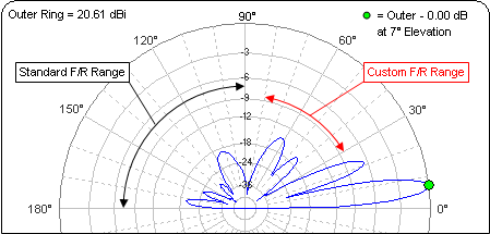
On the Optimize sheet enter the target weights as shown below then enter "30" and "80" as the "Begin" and "End" for the custom F/R range. Be careful to use the "for El slices" range. When you use the range matching the plot type which is currently selected on the Calculate sheet the values and the two Fr/Rear labels will turn red as a reminder. If these fields do not turn red you will not be using a custom F/R range. The current Az/El plot type choice is shown in the log header.
Run the optimizer.
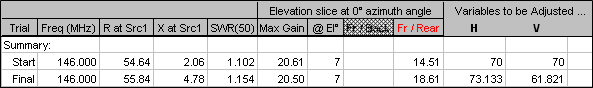
With the target weights you specified, the Gain is essentially unchanged (a minor 0.11 dBi difference) and you reduced the lobes in your custom F/R range by 4.1 dB. If you were displaying the floating pattern window you would see the change already. If not, click the Calculate and Show Pattern button.
Remember, regardless of whether or not you use a custom F/R range for optimization the F/R value which is shown on the Calculate sheet is always for the standard range.
Keep in mind this was only an example to illustrate the use of custom F/R ranges. If minimizing certain lobes really was a design objective you probably would want to optimize the dimensions for a single Yagi first, then combine four of those in a stack and do a second optimization.
Reflector or Director? Are You Smarter than the Optimizer?
Here is a final little example whose real purpose is not to mimic the "Are You Smarter than a 5th Grader?" game show. Instead, it will demonstrate some ways to use various AutoEZ features that might not have occurred to you.
Suppose you wanted to build a 2 element Yagi for the 12 meter band. Should the parasitic element be longer (reflector) or shorter (director) than the driven element? Is there any difference in gain or pattern? How about feedpoint impedance? Let's see.
On the Wires sheet click the Clear All button. Then click Change Units and select meters for wire XYZ coordinates and millimeters for wire diameters. Since there are no wires it doesn't really matter which option you choose in the top of the dialog.
On the Insr Objs sheet change the source placement to Wire #1 50%. We haven't added any wires yet but when we do the source will be in the middle of the first one. If necessary clear any other insertion objects such as loads or transmission lines.
On the Variables sheet again click Clear All and set the Frequency to 24.9 MHz. Define two variables for element lengths, each roughly λ/4, and a third variable to control the spacing between elements, initially set to 1 meter or about 0.08 λ.
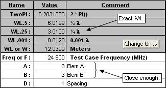
Still on the Variables sheet, click the Stepped Dia button. Use Clear All to remove all existing entries. Enter A for the first section length with a diameter of 25 mm. Enter "0" (zero) for the X coordinate and "0" (zero) for the Z coordinate. Click Create, then change the section length to B and the X coordinate to D. Click Create again and then close the dialog.
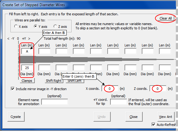
What just happened? Using the dialog was a quick way to create the two elements of the Yagi, with lengths and spacing controlled via variables, without having to even visit the Wires sheet tab. Each element has only a single diameter, sometimes called "mono-taper", so only a single wire is needed. Just because the dialog lets you specify up to 40 wires with 40 diameters doesn't mean you have to use them all.
Now click Optimizer Setup and then Select All. On the Optimize sheet enter 24.9 MHz as the first frequency and clear any other frequencies. Set the targets to the Defaults values but don't start just yet. First let's decide how you might feed this antenna.
From a previous example you saw that if the source resistance was somewhere close to 20 ohms you could shorten the driven element to add some negative reactance, then attach a hairpin in parallel to both cancel the reactance and transform the resistance to 50 ohms. When the driven element length is changed by a small amount it has almost no effect on the gain or pattern. Hence if the source impedance is optimized to roughly 20+j0 ohms you know you could then easily change it (by shortening the DE) to
20–j24.5 ohms, then cancel the reactance with a hairpin and transform it to 50+j0.Where did the
–j24.5 number come from? Here's the equation to get parallel form Rp given series form Rs and Xs.Rp = (Rs^2 + Xs^2) / Rs
You can rearrange the equation to solve for Xs.
Xs = ±SQRT(Rp*Rs - Rs^2)
You want Rp=50 (assuming you want to match to a 50 ohm line) and you know the feedpoint Rs will be 20, hence Xs=±24.5. Since you know the feedpoint reactance will be canceled with positive reactance from the hairpin the correct choice is
Xs=–24.5 .So how do you force the optimizer to search for a feedpoint impedance of 20+j0? Tab to the Calculate sheet and click the small SWR Zo button located just below the thumbnail plot. Change the Zo reference from 50 to 20. That means that the reference for SWR calculations will be 20+j0 so if you optimize on minimum SWR(20) it's the same as shooting for a source impedance of 20+j0. Just what you wanted.
While you are on the Calculate sheet make sure the ground is set to Free Space and the plot type is Azimuth at 0° elevation angle.
Now for the big question. Given your targets of minimum SWR(20) and maximum Gain (in any direction), will the optimizer create a Reflector configuration (element B longer than element A, forward lobe points left) or a Director configuration (element B shorter than element A, forward lobe points right)? Be sure to check the Show Pattern option box so you can see the pattern as the optimizer is running. You know what to do next.
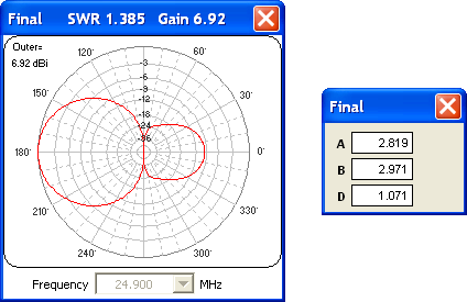
Reflector it is. But remember, that's based on the target objectives you entered. You might try adding a Front/Back or Front/Rear target to the mix, with or without changing the weights. You could also try a different initial spacing. Be sure to click the Reset to Latest Start Values button before each run so you'll always start from the same point, with both elements equal length.
Now suppose you have your heart set on a Director. You can stack the deck in favor of that solution. Just enter "2.9" in place of "3" as the value for B (to start with element B shorter than element A rather than starting with equal lengths) then use the other reset button, Reset to Selected Log Row.
And with that it's time to move on to something else. Don't forget to change SWR Zo back to 50 ohms at some point.
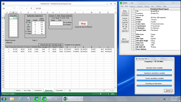
Case Study - 10m Yagi
W8WWV used the optimizer to design a 10m Yagi on behalf of K8AZ. They very kindly gave me permission to pass along the notes made by W8WWV during the design process.
Preliminary report (PDF, 205 KB)
Final report (PDF, 1.02 MB)