- User-Defined Result Columns
- "Subsets" on the Custom Chart
- Exponential Frequency Steps
- "Frequency-Column" on the Custom Chart
- Wire Formulas for a Diamond Shape
- Create Animated GIFs
- Use a "Scratch Workbook"
- Trendlines and Regression Analysis
- Read NEC, AO, NEC/Wires, and MMANA-GAL Files
- Read YM, YS, YO, and YW Files
- Compare Measured vs Modeled with Zplots
User-Defined Result Columns
After you've set up a series of test cases using the left side of the Calculate sheet and done a Calculate, the test case results are shown on the right side of the sheet. Results include R, X, SWR, Max Gain, and so on. But what if you want to calculate, and perhaps plot, some other parameter?
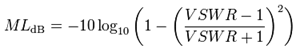
Let's take mismatch loss as an example. As this Wikipedia article shows, one way to calculate mismatch loss is by using SWR.
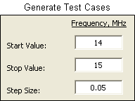
To illustrate the procedure, open BYDIPOLE.ez and generate a series of test cases from 14 to 15 MHz. Don't calculate just yet.
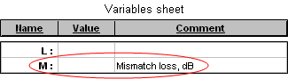
Now pick an unused variable name and give that variable a descriptive comment. Variable name M seems like a good choice in this case.
On the Calculate sheet in an unused "Variable Names and Values" column enter your chosen variable name. In the first test case row enter the formula for your variable. Finally, use the Excel "fill handle" to fill that formula down the page. Any cell references in your formula will be automatically adjusted for each test case row. That is, "I11" in the initial formula will be automatically changed to "I12" in row 12, to "I13" in row 13, all the way down to "I31" in row 31.
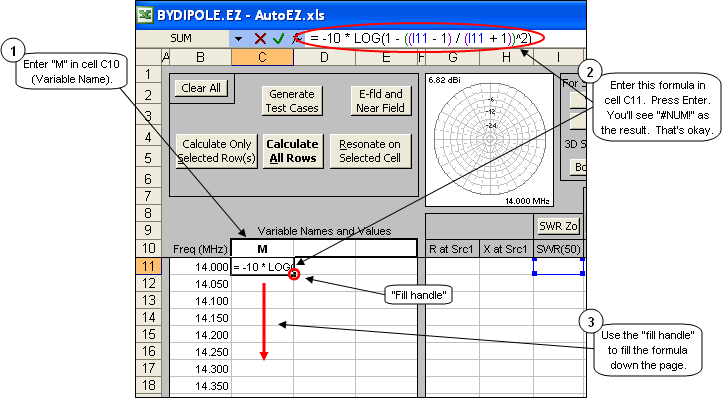
In this particular example, since SWR has not yet been calculated and hence has a default value of zero, the formula initially evaluates to
"= -10 * LOG(0)" . Since "LOG(0)" is not valid the result is the Excel error code "#NUM!". That's fine, the formula will be re-evaluated after the SWR column has been filled in.You don't have to use all the extra blank spaces in the formula. I just did that to make the formula easier to read. Remember to not put a space before the "=" sign.
Now when you Calculate All Rows AutoEZ will, for each row, build a model and send that model to EZNEC. EZNEC will run the model through the NEC engine. AutoEZ will read and parse the output file from EZNEC and put the SWR value in column I. And Excel will use your formula to calculate the mismatch loss in column C.
Calculate and then tab to the Custom chart sheet. Change the Y axis selection to
"Variable 1" (your M variable) and the X axis selection to"Frequency-Line" .
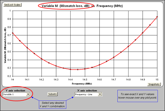
And that's how you create and plot a user-defined result column. If desired you could use the Main & Axis Titles button to change the title text from "Variable M (Mismatch loss, dB)" to just "Mismatch loss (dB)" or whatever suits your needs.
Other formulas that might be useful:
Note that reflection coefficient magnitude and return loss are shown in the "Test Case" information frame on the Smith sheet and are also available as drop-down plot choices on the Custom sheet, so there is usually no need to calculate these parameters as user-defined results. Also note that return loss is a positive number but is plotted as a negative number on the Custom sheet.
- Impedance magnitude (|Z| or Zmag):
=SQRT(G11^2 + H11^2)
- Impedance angle (θ or theta):
=DEGREES(ATAN2(G11, H11))
- Quality factor (Q):
=ABS(H11)/G11
- Source resistance, parallel form (Rp):
=(G11^2 + H11^2)/G11
- Source reactance, parallel form (Xp):
=(G11^2 + H11^2)/H11
- Source inductance, μH (LμH):
=H11/(TwoPi * B11)
- Source capacitance, pF (CpF):
= -1000000/(TwoPi * B11 * H11)
- Reflection coefficient magnitude (ρ or rho):
=(I11-1)/(I11+1)
- Return loss, dB (RL):
=-20 * LOG((I11-1)/(I11+1))Remember, C and R cannot be used as variable names since those two letters are reserved for Excel internal use to identify Columns and Rows on a sheet.
"Subsets" on the Custom Chart
In the previous example perhaps you noticed the Subsets button on the Custom sheet tab. What's that all about? Here's an example.
Once again, start by opening BYDIPOLE.ez. On the Wires sheet use the Move/Copy button and specify a Z axis offset using variable H. On the Calculate sheet make the following test case entries.
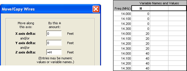
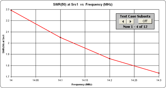
What you have requested is a frequency sweep from 14 to 14.3 MHz with the antenna at a height of 30 feet (Z offset 0 from the original height of 30 ft), followed by a sweep over the same frequency range but with the antenna at a height of 50 feet (Z offset 20 from the original height), followed by another sweep with the antenna at a height of 70 feet (Z offset 40 from the original height).
Calculate and tab to the Custom sheet. Change the Y axis selection to
"SWR at Src" .
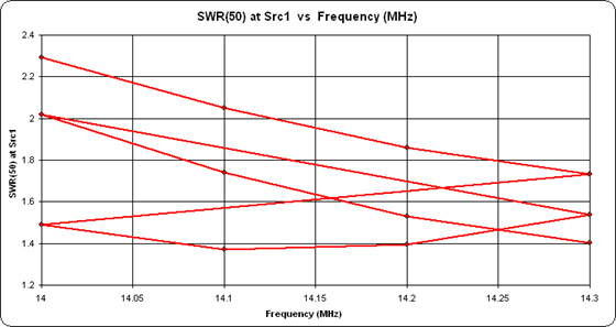
Obviously this is not a very useful chart. It shows exactly what was asked for, namely Frequency on the X axis and SWR on the Y axis. But because the same set of frequencies is repeated three times on the Calculate sheet, the plotted line shuttles back and forth across the page. What is needed is a way to plot just the points for one complete frequency sweep without plotting the other sweeps. The Subsets button allows you to do that.
Return to the Calculate sheet. Select just that set of rows that represents one complete subset of the calculations, in this case one frequency sweep. Note that it doesn't matter what column you select and you need not select the first subset of rows.
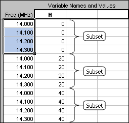
Now return to the Custom sheet and click the Subsets button.
The chart will now show just the data from the subset of rows selected on the Calculate sheet. In addition, a spinner will be available to make it easy to cycle through the other same-sized subsets of data. You can return to the Calculate sheet at any time and you will find that the subset of rows currently being plotted is now also selected, making it easy to correlate between a plotted subset and the corresponding rows.
If desired you may take a snapshot of the plotted points for one subset and compare that to the plot for a different subset.
As you cycle through the subsets you may notice that the chart scales will automatically change to accommodate only those plotted points that are shown at any one time. This is advantageous in that it allows any particular set of points to expand over a larger region of the chart. However, there may be times when you want to lock a chart scale to make it easier to compare the relative plotted position of one subset versus another. To lock a chart scale use the
Set/Lock Scales button.Caution: The scale will remain locked until you use the button again and return to auto-scaling. That means that if you decide to plot a different parameter on the Y axis, the plotted points may not show because they are entirely "off-scale." This can be confusing if you are not expecting it. It is up to you to remember to return to auto-scaling when you no longer want the scale to be locked at a particular min and max value.
Exponential Frequency Steps
When modeling over a wide frequency range, say 1 to 100 MHz, sometimes you might want to use exponential instead of linear frequency steps. Here's how to do that.
Rather than have a fixed linear step size, such as 0.25 MHz, the basic idea is to first define an exponential step size.
ExpStep = (Log(LastFreq) - Log(FirstFreq)) / (NumSteps - 1)Once you've picked a value for "FirstFreq" the subsequent frequencies can be calculated as follows.2nd Freq = 10 ^ (Log(FirstFreq) + 1 * ExpStep)When the definition for "ExpStep" is combined with the formula for the Nth frequency you have:3rd Freq = 10 ^ (Log(FirstFreq) + 2 * ExpStep)
Nth Freq = 10 ^ (Log(FirstFreq) + (N-1) * ExpStep)
Nth Freq = 10 ^ (Log(FirstFreq) + (N-1) * (Log(LastFreq) - Log(FirstFreq)) / (NumSteps - 1))So let's apply this to the frequency steps on the Calculate sheet, with the assumption that the first frequency will be 1 MHz, the last frequency will be 100 MHz, and the number of frequency steps will be 25. Open, what else, BYDIPOLE.ez. On the Wires sheet use the AutoSeg button to assign 40 segments per wavelength, odd. That way as the frequency changes over the full range from 1 to 100 MHz the single wire of the model will always have the same segmentation density although a different number of segments for each test case.On the Calculate sheet enter "1" as the first frequency in cell B11. Then select cell B12, the second frequency, and enter the following string in the formula bar at the top of the Excel window.
= ROUND(10 ^ (LOG(B$11) + (ROW()-11) * (LOG(LastFreq) - LOG(B$11)) / (NumSteps - 1)), 3)Hint: You can swipe the above line on this web page, press Ctrl-C to copy, return to the Excel window, select cell B12, click on the formula bar to activate it (or just press F2), then press Ctrl-V to paste. (If you neglect to click on the formula bar or press F2 you will paste both the text characters and the text font, not what you want.) Change "LastFreq" to 100 and "NumSteps" to 25, then press Enter. If you press Enter before changing "LastFreq" and "NumSteps" the formula will evaluate to the Excel error code "#NAME?" meaning you used an undefined name in the formula. That's not a catastrophe, just revise the formula to replace the undefined names "LastFreq" and "NumSteps" with the desired numeric values of 100 and 25.That sets the second frequency. Now use the "fill handle" to fill the B12 formula down the page until you reach cell B35 which will be 25 steps. When you release the mouse button the final frequency will be 100 MHz, as desired.
How does this work? "LOG(B$11)" is "Log(FirstFreq)". The "$" sign forces the cell reference to stay as B11 as the formula is filled down the page. Without it the B11 would change to B12, then B13, and so on, not what you want. "ROW()" is a built-in Excel function that returns the current row number, so when
"ROW()-11" is used in a formula on row 12 the result is "1", when used in row 13 the result is "2", and so on. Hence"ROW()-11" is the equivalent of"N-1" . Finally, the outer"ROUND(..., 3)" rounds the calculated frequency to the closest KHz.Now why on Earth would you go to all this trouble? Calculate and tab to the Custom sheet. Change the Y axis selection to "Slice Max Gain".
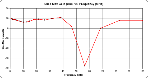
Notice how the frequency steps are "bunched up" on the low end of the scale. Now click the
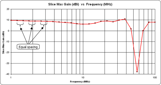
Set/Lock Scales button and check the "Logarithmic" option for the X axis.
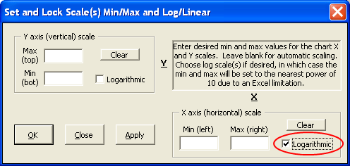
Now the frequency steps will be "evenly spaced" across the entire range.
If you are using Excel 2007 or later the restriction shown in the dialog window about the scale min and max being set to the nearest power of 10 does not apply. However, if you choose "non power of 10" values for the min and max the vertical (frequency) gridlines will have unusual values and be very difficult to interpret.
"Frequency-Column" on the Custom Chart
Sometimes when modeling a multi-band antenna you may use frequency steps that are neither linear nor exponential but instead are discrete frequencies in each band. In that case there's a feature of the Custom sheet that may come in handy.
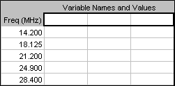
Open sample model "Diamond Pentaband Quad.weq". For this model the frequency steps are defined like this.
Calculate and tab to the Custom sheet. If necessary clear the "Logarithmic" option for the X axis from a previous example.
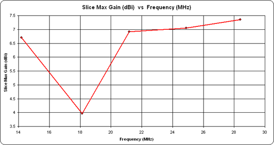
Now there's nothing particularly "wrong" with this chart but it doesn't do a very good job of highlighting the "separate bands" nature of the frequency steps. So change the X axis selection from
"Frequency-Line" to"Frequency-Column" .
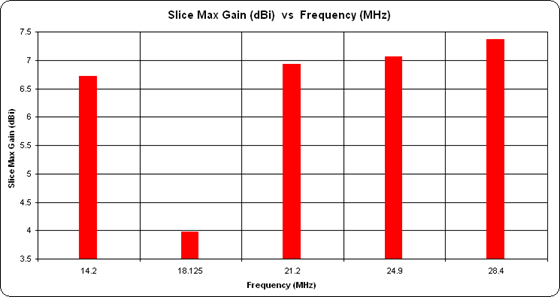
That's better. Now it is obvious that the frequencies are discrete values rather than a continuum.
Wire Formulas for a Diamond Shape
Throughout the AutoEZ documentation you've seen countless examples of how to create square loops. You've also seen an example of how to create a Delta Loop. However, for mechanical support reasons many loops are built in a diamond configuration. The feedpoints are typically in a corner instead of midway along a straight wire. Here's how to create diamond loops.
Open sample model "Diamond Pentaband Quad.weq".
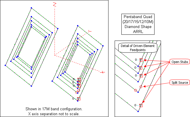
This antenna has the same dimensions as the square Pentaband Quad described earlier. And like that earlier antenna it also includes portions of the feed system in the form of open-circuit stubs.
Don't let the viewing perspective fool you. All four sides of each loop are the same length. The source is an EZNEC "split source" (type SI) which is specifically designed to be used when a source must be placed at a
2-wire junction, in this case 0% along the first wire of a loop and 100% along the fourth wire.Unfortunately there is no such thing as a "split" transmission line. Without "breaking" the loop to add a short wire between the two ends the best that can be done is to place the stub at the start of the first wire of each loop and then use a sufficiently large number of segments such that each segment is very short. That way the stub will be "almost" at the corner junction.
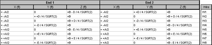
The same variables with the loop circumferences are used as with the square Pentaband Quad model but the wire XYZ coordinate formulas are based on the "Basic Dimensions" of a diamond.
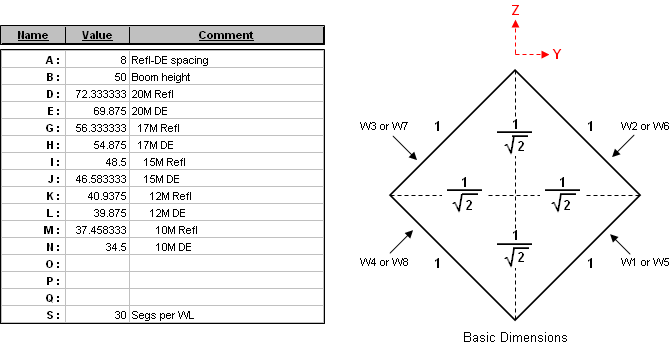
In the above "Basic Dimensions" view the loop circumference is 4 units. Each side is therefore length "4/4" or 1 unit. To convert that diagonal length of 1 to a ±Y or ±Z coordinate requires a division by SQRT(2). Hence if the actual loop circumference is D units the formula for the coordinate is "±D/4/SQRT(2)" instead of "±D/8" as was used for the square shape. So, for example, the 20M reflector (wires
1-4 ) and driven element (wires5-8 ) loops are defined like this.
Again, extensive use of the "W#E#" type shortcut makes it easy to define the first loop, then Copy/Paste (to duplicate 4 rows) and Edit/Replace (to change variable names) makes the task a lot less daunting than it seems. And with today's computers the fact that the "4/SQRT(2)" factor is evaluated 80 times (40 wires times 2 ends) is completely inconsequential.
An alternative method to create the wires of the model would be to use the AutoEZ Create Wires - Loop function. In that case AutoEZ will take care of all the trigonometry under the covers. The only thing you have to do is define the variables for the loop dimensions.
Create Animated GIFs
On many of the AutoEZ web pages you've seen examples and illustrations that make use of animated GIFs. Perhaps you'd like to create something similar for your own antennas on your own web pages. Here's how.
To create an animated GIF you need: 1) A set of two or more individual GIF format files that serve as the "frames" for the animated GIF "movie", and 2) Software than can assemble these separate files into one animation.
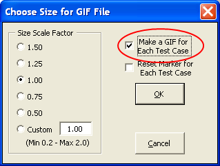
Still using the calculated results for the "Diamond Pentaband Quad.weq" model from the previous example, tab to the Patterns sheet. Click the Make GIF button. In the dialog that pops up select the "Make a GIF for Each Test Case" option.
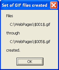
When you click OK AutoEZ will cycle through all the test cases, starting with number 1, and create a GIF for each with a sequential temporary name. The path will be whatever you used the last time you created a single GIF, so you may wish to create a single file beforehand just to pre-set the path.
Now you have the frames of the movie. For the second step you'll need a separate "GIF Animator" program. The one that I have used for many years is GIF Construction Set Professional by Alchemy Mindworks. Another nice program is Easy GIF Animator by Blumentals Software. Both of these programs are very reasonably priced. (I have no affiliation with either company.) If you're looking for "free" as opposed to "low cost" you can find several recommendations at this gizmo's freeware page.
Update: Here's a very handy online animated GIF maker.
No matter which program you decide to use there will be a bit of a learning curve. However, in short order you'll be producing animated GIFs like this.
(Press Esc to stop the animation, F5 to restart.)For this example I used a Size Scale Factor of 0.75. Before making the GIF files I froze the outer ring at 7.36 dBi, the Max Gain at 28.4 MHz, so that the gain difference at each frequency step would be obvious. Use of the "Reset Marker for Each Test Case" option wasn't applicable here since the max gain was always at 0° azimuth angle. You might want to use that option for elevation slices where the angle of the max gain point varies.
The option to make a set of GIF files is also available on the Smith and Currents sheet tabs.
Use a "Scratch Workbook"
The scratch pad area on the Variables sheet tab comes in handy for lots of different uses but one major drawback is that it doesn't persist between models. The scratch pad area is saved as part of the .weq file for any given model, so each time you open a new model the scratch pad area is replaced. What if you want to save data or calculations "between" models?
You can create a "scratch workbook" and use that instead. Just press Ctrl-N (N is for "new workbook"). That will open a new, blank workbook typically named Book1. The new workbook will show as a separate icon in the Windows taskbar.
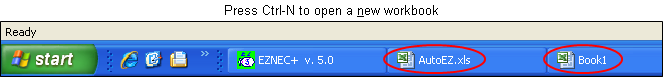
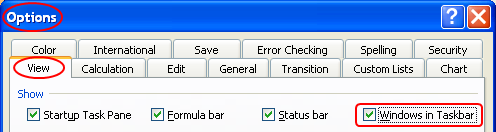
If you don't see a new icon you can adjust the Excel options in order to make it appear. With Excel 2003 and earlier click Tools > Options on the Excel menu bar. In the Options dialog select the View tab then select the "Windows in Taskbar" option.
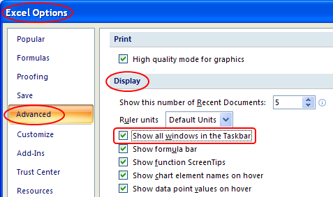
With Excel 2007 click the large "Office" button and then the "Excel Options" button. With Excel 2010 click the "File" menu and then the "Options" button, just above the "Exit" button. In the Excel Options dialog select Advanced then scroll down to the Display section and select the "Show all windows in the Taskbar" option.
Windows 7: Even with the above option changes you may still see only a single Excel taskbar icon. You can hover over that icon and make a choice to switch to a different workbook, or you can change the way taskbar icons are shown as explained in this PCWorld article.
By clicking on the corresponding taskbar icon (or perhaps hover and choose) you can switch back and forth at will between AutoEZ and the new workbook and you can do Copy/Paste operations between the two. If desired you can save the new workbook to preserve anything you might have put in it.
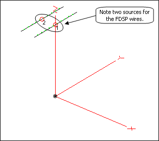
One typical use for a "scratch workbook" would be to copy a group of wires from one model to another. Here's an example. Using AutoEZ, open EZNEC sample model FDSP.EZ. The EZNEC samples are typically found in "C:\Program Files [(x86)]\EZW\Ant". (The "(x86)" part will be present on
64-bit machines.)
On the Wires sheet select cells B10 through I12 and press Ctrl-C to copy. Then press Ctrl-N to open a new workbook if you haven't done so already. If you want to paste cell formatting (font sizes, number of decimals, vertical separator lines, etc) as well as cell values press Ctrl-V. If you want to paste only the cell values, which is probably the better choice in most situations,
right-click on the target destination cell (such as cell A1) and then select Paste Special - Values. AutoEZ will show a brief message about this the first time you copy "out of" the AutoEZ workbook.
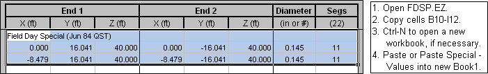
Now return to AutoEZ and open EZNEC sample model BYVEE.EZ. Switch back to Book1 and copy the cells you previously pasted. The group of cells will probably still be selected so all you have to do is press Ctrl-C. Switch back to AutoEZ,
right-click on cell B14 and select Paste Special - Values.
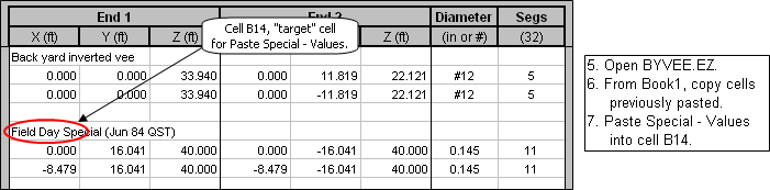
Now let's see what we've got.
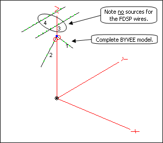
What happened to the two original sources for the FDSP wires? Well, all you did was copy out and then paste back in the wires of the FDSP model, not the wires and the sources. Using a scratch workbook in the manner just described is similar to the EZNEC "Importing Wire Coordinates" feature. It is not the same as the EZNEC "Combining Antenna Descriptions" feature. (You can find both those terms in the EZNEC Help.)
Things get a little trickier when you want to transfer wires between .weq format models rather than .ez models. If you have defined any wire XYZ coordinates using formulas and variables you'll want to Paste Special - Formulas instead of Paste Special - Values. And it's up to you to resolve any duplicate use of the same variable names between the two different models.
Also, if you have used the AutoSeg button to put a formula in the "Segs" column, and your Copy includes the "Segs" column, when you Paste Special - Formulas to Book1 you'll see "#N/A" for the segment count cell(s). This is normal. Then when you Paste Special - Formulas back into AutoEZ you'll see this Excel message.
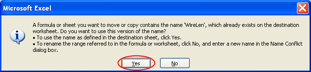
Answer "Yes" to the question.
You'll definitely want to experiment with simple models before you try to transfer dozens or hundreds of wires. If you feel lost at any point you can just close both AutoEZ and Book1 without saving. And if you somehow manage to corrupt the AutoEZ workbook you can always run the installer program (Setup.exe) again to reinstall the entire package.
Trendlines and Regression Analysis
A Trendline is Excel's term for doing regression analysis on the data shown on a chart. Although you can add a trendline manually, AutoEZ has some features to make the process easier.
To illustrate, open good ol' BYDIPOLE.ez again and generate a series of test cases from 14 to 15 MHz.
Calculate and tab to the Custom sheet. Change the Y axis selection to
"SWR at Src" and make sure the X axis selection is"Frequency-Line" and not"Frequency-Column" . Click the Add button in the "Trendline" frame.
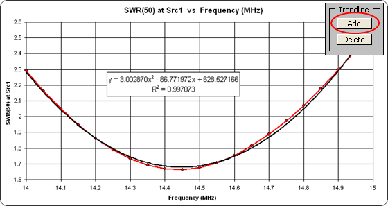
AutoEZ will create a second-order polynomial trendline and show the matching equation and the R2 value. R2 is a measure of the "goodness" of the curve fit; the closer R2 is to 1.0, the closer the trendline trace is to perfectly matching the trace of the original data. If R2 is close to 1.0, as it is in this example, then the equation can be used to both interpolate and extrapolate other Y axis values given any arbitrary X axis value.
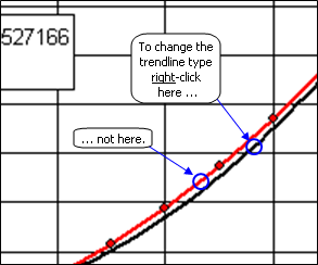
A second-order polynomial trendline turned out to be a good choice in this case but, depending on the shape of the original trace, other choices may be more suitable. To change the trendline type,
right-click on the black trendline. Make sure you point to the black trendline trace and not the red primary trace.
What you see next will depend on which version of Excel you are using.
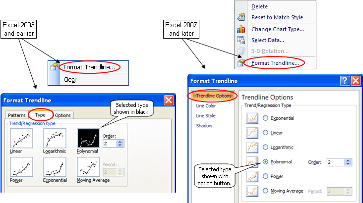
With earlier versions of Excel you can click on one of the other large squares to change the type, or leave the type as polynomial but change the order. Click OK to see the change on the chart. With later versions of Excel the changes are interactive. When you make a new selection or change the polynomial order, the trendline, the equation, and the R2 value will all change immediately.
Although it is fun to generate different types of trendlines for different sets of data, to do anything useful you need the coefficients of the equation for use in other Excel formulas. You could of course manually transcribe the numbers but that's prone to error. To illustrate two better techniques let's first copy the X axis data (Frequency) and Y axis data (SWR) to a scratch workbook.
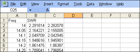
Press Ctrl-N to open a new, blank workbook. Enter two column headers, "Freq" in cell A1 and "SWR" in cell B1. Back on AutoEZ, tab to the Calculate sheet, drag through all the Freq cells
(B11-B31) , press and hold the Ctrl key, drag through all the SWR cells(I11-I31) , then press Ctrl-C to copy the entire multi-column selection at one time. Over to Book1, right-click on cell A2 and select Paste Special - Values.Back to AutoEZ, tab to the Custom sheet. Click once on the border of the equation box to activate the box, then drag through the entire equation but not the R2 value. The selected text will have a dark background. Press Ctrl-C to copy the text.
Important: After you've copied the text, click outside the entire chart. That tells Excel that you are done working (in this case copying) within the chart and now want to do things at the workbook level.
Back to Book1, select cell C2 but don't paste yet. Instead, click in the formula bar (or press F2), then Ctrl-V to paste. (If you paste without first clicking the formula bar or pressing F2, Excel is likely to parse the copied text into several adjacent cells. That's not what you want.) Then make the following changes to transform the copied text into a valid Excel formula.
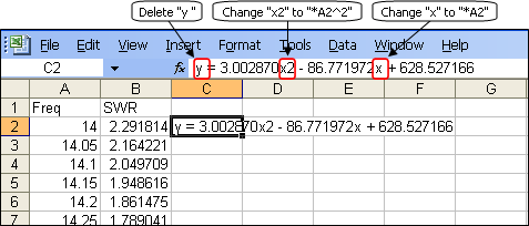
Make sure you don't leave a space before the "=" sign. Press Enter, then use the fill handle to fill the formula down to cell C22.
There are two reasons why the values from the trendline equation are not exactly the same as the original SWR data values: 1) the R2 was not exactly 1.0 meaning the trendline was not exactly superimposed on the trace of the original data, and 2) the equation showed the coefficients to only 6 decimal places.
The second technique to get the coefficients, which produces results with 15 digit double-precision, is to use the Excel LINEST function. Very briefly, here's the process. In three spare cells, say
F2-F4, enter these formulas:=INDEX(LINEST(B2:B22, A2:A22^{1,2}), 1, 1)Note that the "{1,2}" portion is in braces, not parenthesis. The formulas will evaluate to:
=INDEX(LINEST(B2:B22, A2:A22^{1,2}), 1, 2)
=INDEX(LINEST(B2:B22, A2:A22^{1,2}), 1, 3)
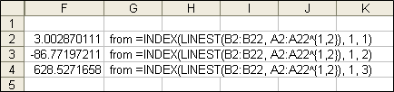
Although displayed with only 10 digits, under the covers all three results are 15 digits long (which may or may not make any practical difference). So instead of doing a copy/paste of the text in the trendline equation box you could use the LINEST function to obtain the coefficients. Different trendline types use different forms of LINEST or different Excel functions all together. For more details see the Walkenbach page referenced below.
Additional information on trendlines and regression analysis:
Or search for "Trendlines" using the Help function for your version of Excel.
- Trendline Fitting Errors by Jon Peltier
- Trendline Coefficients and Regression Analysis by Tushar Mehta
- Chart Trendline Formulas by John Walkenbach
Read NEC, AO, NEC/Wires, and MMANA-GAL Files
The Open Model File button, found on the first four sheet tabs, is typically used to read AutoEZ format (.weq) or EZNEC format (.ez) files. However, you can also open NEC format (.nec or .inp), AO format (.ant), and
MMANA-GAL (.maa) files as well. AO is short for Antenna Optimizer by Brian Beezley, K6STI. The .ant file format is also used by the K6STI NEC/Wires program.There are certain restrictions and limitations when reading these file types. For NEC files:
AutoEZ processes only GW cards for the structure geometry. Any GA (arc), GH (helix), SP (patch), and other such cards are ignored with an appropriate warning message. Use of absolute segment numbers on EX, LD, and TL cards is not supported. The file must not contain a mixture of LD4 cards (type R±jX loads) and LD0/1 cards (series or parallel RLC loads), although any combination of LD0 and LD1 is allowed. If the file contains more than one LD5 card (wire loss) AutoEZ will use the last one found. NT cards are ignored except as used to create "current" sources. Certain other limitations also apply.For K6STI AO and NEC/Wires files:Note that NEC files produced by
NEC-Win Plus+,NEC-Win Synth, 4nec2, and the 4nec2 Build utility can usually be read without any problems. Any 4nec2 "SY" (symbol) cards will be converted to AutoEZ variables and formulas.Symbols will be converted to AutoEZ variables and formulas.For MMANA-GAL files:As with NEC files, AutoEZ does not support a mixture of R±jX and RLC type loads. Laplace loads are not supported. The Symmetry option is ignored.
If a source, load, or transmission line is placed in the "center" of a wire, AutoEZ will automatically insure that the wire has an odd number of segments. Some manual adjustments may be necessary if sources or loads have been placed at positions other than the beginning, end, or center of a wire.
Shift and Rotate commands are not supported directly but a comment line will be shown on the Wires sheet with instructions on how to accomplish the same thing using the AutoEZ Move/Copy and Rotate buttons.
Files may contain a "taper wire set" section. AutoEZ will interpret both the "master" wire and the associated taper schedule to produce a set of "real" wires."S" type (Laplace) loads are not supported.
Segmentation information is ignored. All wires are initially set to 20 segments per wavelength. You can use the AutoEZ AutoSeg button to change the segmentation density if desired.
Any "pulse offset" for sources or loads (such as "w1c3") is ignored. You may have to manually adjust the placement of such items.
Any "stack" specification is ignored. You can use the MMANA-GAL "Edit > Make Stack > Make new ..." sequence to include all wires in the file.
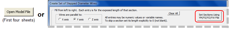
Read YM, YS, YO, and YW Files
As of maintenance release v2.0.25 AutoEZ can read files created by the DXE Yagi Mechanical program (YM, file type .stm); the K7NV Yagi Stress program (YS, file type .ys2); the K6STI Yagi Optimizer program (YO, file type .yag); and the N6BV Yagi for Windows program (YW, file type .yw). These files may be read via the normal Open Model File button or via the Create Stepped Diameters dialog window. The latter makes it especially convenient to assign variables for element tip lengths and/or boom positions in order to experiment with changes to the model.
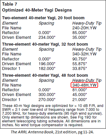
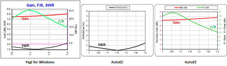
The "HF Yagi Arrays" chapter in recent editions of The ARRL Antenna Book describes many different Yagi configurations. Yagi for Windows format model files (.yw) are contained on the CD that is bundled with the book. For example, the book describes three 40-meter Yagis.
Note that many of the Yagi for Windows (.yw) and Yagi Optimizer (.yag) models have a "boom clamp" as the first taper section. When such models are read via the Open Model File button the boom clamp will be removed automatically and the length of the second taper section will be incremented as necessary. This yields much better Average Gain Test values along with calculated results that are closer to those shown by the YW program. To illustrate, with model
"340-48H.YW" as shown above:
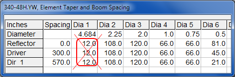
The 12" length of the 4.684" equivalent diameter clamp will be added to the 108" length of the 2.25" diameter second taper section.
If you want to include the boom clamp in the model, read the file using the Create Stepped Diameters dialog rather than the Open Model File button. And if you want to use the Create dialog and eliminate the boom clamp, manually add the length of the first taper section to the length of the second taper section then use the Shift Left button on the dialog window to eliminate the first section.
Also note that many Yagi for Windows (.yw) and Yagi Optimizer (.yag) models require that a hairpin be added at the feedpoint. In many cases the properties for the hairpin will be shown in the comments for the model. Look on the Wires sheet below the last wire row. Again with model
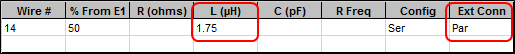
"340-48H.YW" as an example:
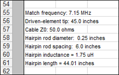
You could model this hairpin as a 1.75 µH (or whatever the comment shows for inductance) RLC type load with a parallel external connection.
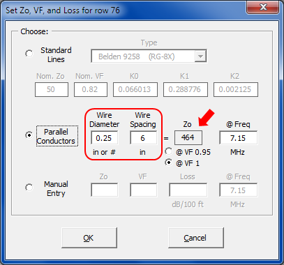
Or you could model it as a shorted stub transmission line. First use the Set Zo, VF, and Loss button on the
Insr Objs sheet to determine the characteristic impedance Zo for two parallel 0.25 inch diameter wires separated by 6 inches (or whatever the comment shows for hairpin rod diameter and spacing).
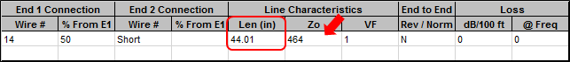
Then add a shorted stub transmission line with that Zo value and with a length 44.01 inches (or whatever the comment shows for length).
A hairpin match is typically required if the unmatched feedpoint impedance is approximately
25-j25 ohms (plus or minus several ohms for both R and jX) at the design frequency. If a hairpin is required but no specifications are included with the model, a good first estimate is that the hairpin must provide about +50 ohms of reactance at the design frequency.To convert that reactance value to a load inductance or shorted stub length, first set the "Freq" cell (cell C11 on the Variables sheet) to the design frequency, 7.15 MHz in this example. Setting "Freq" will automatically set the "WL" (wavelength) read-only variable. Then to determine the inductance in µH enter the following formula in a spare cell of the scratch pad area:
=50 / (TwoPi * Freq)Or to determine the length of a hairpin shorted stub transmission line having an assumed Zo of 464 ohms, use this formula:At 7.15 MHz a reactance of +50 ohms equates to about 1.11 µH of inductance. Don't forget that the load must have a parallel external connection, Ext Conn "Par".
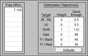
=ATAN(50 / 464) / TwoPi * WLAfter an initial estimate of the load inductance or transmission line length is calculated you can use the optimizer to find a more exact value. Use a variable for the value of the load inductance or the length of the shorted stub transmission line. Optimize on that variable name and use a target weight of 1 for SWR and zero (or blank) for all the other weights.At 7.15 MHz a reactance of +50 ohms equates to about 28.2 inches of near-ideal shorted stub transmission line with a Zo of 464 ohms. Note that the ATAN function returns an angle in radians, not degrees.
With model
"340-48H.YW" the optimized inductance will be about 2.4 µH and the optimized shorted stub length will be about 60 inches (using the NEC-2D engine). But the minimum possibleSWR(50) will be 1.4. If you want to get a perfect match to 50 ohms, and hence improve thelow-SWR bandwidth, you'll need to optimize on the hairpin inductance or stub length and on the length of the driven element. Doing that two-variable optimization will result in an inductance of 1.46 µH or a shorted stub length of 36.9 inches combined with a tip section length of 39 inches.So why don't those hairpin and tip length values match what is shown in the comments for model
"340-48H.YW" ? The comments are based on an unmatched feedpoint impedance of35.6-j19.4 ohms as calculated by the Yagi for Windows program. YW is a special-purpose program designed strictly for monoband Yagis. It uses neither the NEC nor MiniNEC calculating engine. On the other hand, using the EZNEC NEC-2D engine and with the tip length at 39 inches as opposed to 45 inches, the unmatched feedpoint impedance is31.7-j24.2 ohms. Hence the hairpin must have a different reactance value in order to match to 50 ohms.Regardless of these relatively minor differences the overall performance of the model is remarkably similar between YW and AutoEZ as shown below.
Additional information on hairpin matching:
Also see section "Element Lengths - Element Spacing - Hairpin Match with 20M5ELYA.ez" on the AutoEZ Using the Optimizer page. In that section, scroll down to the paragraph beginning with "Now for the hairpin match" or just use your browser's Find function to search for the word "hairpin".
- How Shall I Feed the Antenna? by W4RNL
- The "Hairpin" Match by N6MW
Zip files containing dozens of Yagi Optimizer (.yag) models may be downloaded from the ARRL Antenna Modeling Files page. Some of those are predecessors or duplicates of the Yagi for Windows (.yw) models on the CD of The ARRL Antenna Book as mentioned above.
Compare Measured vs Modeled with Zplots

The Zplots Excel application allows you to plot impedance and related data obtained from a variety of sources. As with AutoEZ, Zplots has a Snapshots feature so you can compare one set of data against another. One source of data might be measurements made with any number of different instruments such as the AIM4170, the N2PK VNA, the miniVNA PRO, the DG8SAQ VNWA, and other such devices.
For modeled impedance data, to be used in comparison against actual measurements, you can use the Save as Zplots File button on the AutoEZ Smith sheet tab. That will create a file of the latest calculation results which can be read by Zplots.
To make meaningful comparisons between measured and modeled it is important that you keep in mind the reference plane of your measuring device. For example, if your AutoEZ model has calculated impedance values at the center of a dipole 30 ft in the air then your measurements should be at that same point, not at the lower end of 30 ft of transmission line. As explained in Appendix 1 of the Zplots documentation:
The most accurate way to make antenna measurements is to temporarily disconnect the far end of the transmission line from the antenna, place OSL (Open-Short-Load) terminations at the far end, connect the shack end of the line to your instrument, and perform a calibration. This will move the reference plane of your instrument to the antenna feedpoint, effectively "calibrating out" the transmission line. Then reconnect the feedline to the antenna and make measurements over the frequency range of interest. Readings you make at the shack end of the line will then be the same as if you had made them directly at the antenna.