A very common scenario is the need to make accurate antenna measurements with the antenna system in its operating position, perhaps atop a tower, while the measuring equipment is on the ground. In this situation there is a trade-off between convenience and accuracy. The following techniques may be employed, listed in the order of most accurate to least accurate.

1. The most accurate way to make antenna measurements is to temporarily disconnect the far end of the transmission line from the antenna, place OSL (Open-Short-Load) terminations at the far end, connect the shack end of the line to your instrument, and perform a calibration. This will move the reference plane of your instrument to the antenna feedpoint, effectively "calibrating out" the transmission line. Then reconnect the feedline to the antenna and make measurements over the frequency range of interest. Readings you make at the shack end of the line will then be the same as if you had made them directly at the antenna.

2. The next most accurate technique is to mathematically "subtract out" the effect of the feedline. Note this isn't quite the same as "calibrating out" the feedline since you are using a model of the feedline rather than an actual set of measured responses.

   Perhaps you have a section of the same line that was left over from your antenna installation. If so, you can use the Zplots "Measure Transmission Line Parameters" feature (described on the main Zplots web page) to determine the electrical characteristics of the line: nominal Zo, nominal VF, and loss coefficients K0/K1/K2. Then the only additional piece of information needed is the physical length of the actual antenna feedline.

   If you can terminate the line with either a short or open (one or the other), you can determine the length by using either a) the "unwrap Smith chart" technique (most accurate) or b) the "quarter-wave or half-wave points" technique (less accurate). Both of these methods are described in more detail below. To provide an open circuit termination you can just unscrew the feedline connector at the antenna. If the connector is wrapped in several layers of Coax-Seal, or if the feedline is directly attached to the antenna such as with coax pigtails soldered to either side of a dipole, just place a jumper across the antenna feedpoint to provide a short circuit termination. Make the jumper as short as possible.

   With the electrical characteristics and the physical length in hand, reconnect the far end of the line to the antenna (or remove the jumper) and run a sweep over the frequency range of interest. Load the sweep data into Zplots and then use the "Subtract Transmission Line" feature (described on the main Zplots web page) to "subtract out" the effect of the feedline.

3. If you can't measure the electrical characteristics for an identical section of line you can use an estimate of the characteristics. Zplots contains built-in characteristics for approximately 100 different line types. At least one of them is probably very close (although not exactly the same) as your feedline. Then, as above, determine the physical length of the actual line and "subtract" it out from measured data.

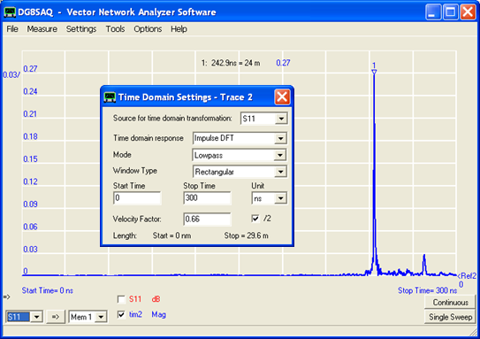
4. Finally, suppose you have the electrical characteristics, either measured or estimated, but you can't access the far end of the line. How can you determine the length of the line without being able to put a short or open at the far end? One technique involves Time Domain Reflectometry (TDR), described below.

So it all boils down to how much accuracy you want versus how many different ways (if any) you can terminate the far end of the line. If you can place OSL terminations at the far end just calibrate out the line. That will take full advantage of the error correction algorithms that are part of your instrument's control software. If you can only place an open or short you can determine the length using one of the techniques described below and then use the Zplots "Subtract Transmission Line" feature with electrical characteristics that are either actual (via measurements of a piece of identical line) or estimated (via one of the built-in line types). And if you have no access to the far end of the line you can use TDR techniques to determine the length, although probably not with as much accuracy as with an open or short termination.

---

Line Length via "Unwrap" Smith Chart:

Here's an example of using Zplots to determine the length of a transmission line. In this case an unknown length (estimated to be between 50 and 100 feet) of Belden RG-213 was terminated with an open circuit. A frequency sweep from 1 to 2 MHz with a 0.05 MHz step size was made and the data file was loaded into Zplots.

This is what the Smith chart would look like. The "Dots On/Off" button was used to put a red dot at each discrete frequency of the sweep. In addition, a marker (blue dot) was placed on the 1 MHz point.

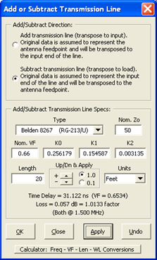
Click the "Add/Subt T Line" button. Choose the "Subtract ..." direction and set the line type to Belden RG-213. The estimated line length is somewhere between 50 and 100 feet so to start set the length to 20 feet and click the "Apply" button. Follow that with lengths of 40 feet and 60 feet. Once the blue dot gets close to the "open circuit" position on the Smith chart (right-hand side, 3:00 o'clock on the outer circle) switch to the "Up/Dn & Apply" spin buttons, first using increments of 1 foot and then increments of 0.1 feet. Alternatively, change from feet to inches; the length value will be automatically converted as necessary. Continue to increment the "subtracted" length until the blue dot and all the other dots are right at 3:00 o'clock. You know that the line was terminated with an open circuit. You have now "subtracted" (mathematically removed) enough transmission such that the Smith chart appears to be an open circuit, even though the measurements were made with a length of line in place. Hence the length that you mathematically subtracted is the actual length of the line. In this example the final length was set at 78.6 feet. The following "time lapse" shows what the Smith chart would look like with varying amounts of transmission line subtracted.

In the example above all the dots ended up on top of one another. But this was a theoretical case shown just to illustrate what it means to "unwrap" a Smith chart. Using "real world" data the situation won't be quite so simple.

This Smith chart shows actual measurement data from approximately 40 feet of Radio Shack RG-58 terminated with an open circuit. The sweep was done from 10 to 50 MHz with fairly tight spacing. You can see that the trace is not perfectly smooth, representing noise or other anomalies in the measured data. The following sequence shows varying amounts of line being subtracted, first in units of feet and then switching to inches.

In this particular case I had determined the electrical characteristics of an identical section of line beforehand using the Zplots "Measure Transmission Line Parameters" feature. The values for nominal Zo, nominal VF, and loss coefficients K0/K1/K2 were automatically transferred to the "User Specified" line type and I continued to use those values, changing just the line length.

If you have not been able to determine the electrical characteristics beforehand, perhaps by measuring a segment of line that is identical to the one running to the antenna, then you'll have to select one of the built-in line types. In that case pay attention to the position of the trace as you near the final "subtracted" length value. The trace may be slightly inside or outside the perimeter of the Smith chart as the two illustrations at left show. That means that the loss characteristics of the built-in line are not quite the same as your line. Try adjusting the K1 and/or K2 coefficients, first by increments of 0.1 units and then 0.01 units, until the entire trace lies on the Smith perimeter. Be sure to wait until you have subtracted almost the correct amount; otherwise, the trace is supposed to be inside the perimeter.

Note: If you change the K1/K2 coefficients be sure to make a note of the new values. That way you can use the same values when you re-attach the line to the antenna, make measurements with the antenna in place, and then again "subtract" the correct amount of line in order to see just the response of the antenna itself. When you make changes to any of the characteristics for the built-in line types those changes are not saved once you close the dialog panel. On the other hand, any changes you make to the characteristics for the "User Specified" line are saved and will be shown the next time you use the dialog.

Also note that it is not necessary to use a large number of points (small step size) when determining the length of a line. Just run a sweep over the frequency range of interest and use enough points, perhaps a few dozen to a hundred or so, to make the "subtraction" steps clear. Using fewer points means that Excel will be able to update the Smith chart faster, something you'll notice when using the "Up/Dn & Apply" spin buttons.

Finally, remember that you could have terminated the line with a short circuit instead of an open circuit. In that case, adjust the "subtracted" length until the trace collapses to the 9:00 o'clock (left side) point on the outer circle of the Smith chart, the short circuit position.

---

Line Length via Quarter or Half-Wave Points:

Another technique used to determine line length is to terminate the line with either an open or short circuit, run a sweep, and then note the frequencies of certain items that are known to repeat every quarter-wavelength of half-wavelength. Commonly used items are impedance magnitude (Zmag) peaks, which repeat every half-wavelength, or impedance angle (Theta) or reflection coefficient angle (Phase) zero-crossings, which repeat every quarter-wavelength.

Here's an example for a section of Belden RG-213 terminated with a short circuit and swept over a range from 20 to 30 MHz. By placing Marker 1 on the first Zmag peak and Marker 2 on the next peak, the marker table will show the frequency difference between the two points. That frequency difference corresponds to a half wavelength. Together with the speed of light and the velocity factor that's all you need to determine what the physical length of the line must be.

You can dig out your pocket calculator. Or you can click the "Add/Subt T Line" button and then click the "Calculator: ..." button near the bottom of the window. (In this case you aren't going to do any "adding" or "subtracting" of transmission lines. It's just that the "Calculator: ..." button is found there.) Choose "Physical Length" as the value you want. Enter whatever frequency difference you got from the marker table, in this example 4.122 MHz. Set the velocity factor to that of the line in question (0.66 in this case) and make sure the electrical length is set to 0.5 wavelengths. Presto, the length of the line is 78.743 feet.

Or is it? If you had started your sweep at 1 MHz the first two Zmag peaks would occur at 2.045 and 6.153. That's a half-wavelength difference of 4.108 MHz which translates to a physical length of 79.011 feet. On the other hand, if you had started your sweep at 90 MHz the first two Zmag peaks would occur at 92.738 and 96.864. That's a half-wavelength difference of 4.126 MHz which translates to a physical length of 78.667 feet.

79.011 feet, 78.743 feet, 78.667 feet. A difference of a little over 4 inches depending on where you start the sweep. What's going on?

The problem is that the velocity factor changes with frequency, as the above chart shows for three different types of coax all having a "nominal" VF of 0.66. For all three the VF approaches 0.66 at very high frequencies. At lower frequencies the amount of change in velocity factor is dependent on the internal inductance of the cable conductors (center conductor and outer shield). The internal inductance is related to the resistance of the conductors. And the resistance of the conductors is related to the loss of the cable. The greater the cable loss (that is, the higher the attenuation in dB/100 ft) the more the VF will change at lower frequencies.

The same concept applies to the time delay of a cable. For example, 100 feet of RG-213 has a one-way time delay of 154.14 nanoseconds at 1000 MHz. But at 1 MHz the same cable has a delay of 155.73 ns. Cables with higher loss would show even more of a difference in the time delay.

This problem does not apply to the "unwrap" Smith chart technique for determining line length. In that case the Zplots algorithm uses the loss coefficients K0/K1/K2 to automatically recalculate the correct VF value for each separate frequency. (Actually the math is a lot more complicated than that but the effect is the same.)

---

Line Length via Time Domain Reflectometry:

Suppose you can't access the far end of the line at all, hence you can't terminate the line with an open or short circuit and use one of the methods discussed above to determine the line length. Using the DG8SAQ VNWA software you have another option for determining the length of a transmission line even when the far end is connected to an antenna. You can take advantage of the VNWA time domain reflectometry (TDR) feature.

Why does this work? For most antennas the feedpoint impedance (that is, the impedance at the far end of the transmission line) will be close to the characteristic impedance of the line only over a relatively narrow frequency range. Or in the case of a multi-band antenna it might be a multiple number of frequency ranges. But if the input end of the line is swept over a very wide frequency range, say from close to DC to a few hundred or better yet a few thousand MHz, at the great majority of those frequencies the terminating impedance will be far removed from the line's Zo. Hence for most of the spectrum the reflection coefficient will be closer to 1 than to 0. (If the line were terminated in an open or short circuit the reflection coefficient would be exactly 1 at all frequencies.) A reflection coefficient close to 1 means that a large part of the energy that is fed into the line will be bounced back at almost all frequencies. When the wide frequency spectrum is converted to the time domain via an Inverse Fourier Transform the response will look like a pulse bounced back from a point on the line where there is a large impedance mismatch; namely, where the line connects to the antenna.

For example, below is what the reflection coefficient magnitude (rho) might look like at the antenna feedpoint for a typical tri-band (20-15-10 meter) Yagi. The frequency sweep is from 1 KHz to 160 MHz. A reference line at rho value 0.333, which corresponds to an SWR of 2:1, has been added. The 20 meter, 15 meter, and 10 meter bands have been marked. You can see that although the reflection coefficient magnitude exhibits a very complicated pattern, at most frequencies the value is relatively high. Hence at most frequencies most of the incident pulse energy will be bounced back.

Note that the amplitude of the returned pulse won't be the same as if the line were terminated in an open or short. In addition to that portion of the pulse energy that is dissipated due to the attenuation of the line, part will be absorbed by the antenna itself. But in this case we don't care about the amplitude; we can use other means (such as measuring a section of identical line and/or using one of the Zplots built-in line types) to get the loss characteristics of the line. All we want is the time delay of the returned pulse which can be converted into a distance.

Now rather than stopping at 160 MHz suppose you widen the frequency span, say up to 1400 MHz. And further suppose you run the sweep at the input end of the transmission line. (Remember, you can't access the far end.) You know that the line is RG-213 with a nominal velocity factor of 0.66 and you estimate the length to be somewhere between 50 and 100 feet. A few mouse clicks with the VNWA program would show something like this, indicating that the line is approximately 24 meters long.

In more detail, use these steps to produce a plot like the one above:

1. Attach the shack end of the line to the TX port of the VNWA device and run a sweep. For best accuracy set the start and stop frequencies to the minimum and maximum allowed values and set the number of points to the max allowed (8192). Be sure to use linear and not logarithmic steps.

   Note: The VNWA software can also be used with the N2PK VNA hardware. And you can use the VNWA software by itself even if you don't have either of the supported hardware devices. In that case, use whatever instrument you do have to run a sweep over the maximum frequency range with a step size that results in no more than 8192 points. Save the sweep data in Touchstone s1p format. (If your control software does not have the capability to produce s1p files you can always load the data into Zplots and then use the "Save as S1P" button.) Then with the VNWA program use File > Import Data > s1p > to S11.

2. Click Settings > Diagrams > Display > Traces. Add a second trace. Select "lin. magnitude" and "Time" for the trace options.

3. Click Settings > Time Domain > Trace 2 (or whatever trace number you just added). In the Time Domain Settings dialog select "S11" for the source, "Impulse DFT" for the response, "Lowpass" for the mode, and "Rectangular" for the window type. Set the Velocity Factor to match the transmission line and be sure the "/2" box is checked. Enter "0" for the Start Time. For the Stop Time enter a value which is high enough such that the "Stop" length (shown in meters) is greater than the estimated maximum length of the line. In the example above the estimated line length is 50-100 feet; 100 feet is about 30 meters and the Stop Time of 300 ns (nanoseconds) gives a maximum line length of 29.6 meters. Assuming the Stop Time is set high enough you should see a very pronounced spike in the trace.

4. Optionally, "uncheck" the original S11 trace just to remove plot clutter.

5. Right-click the time scale label "units per division" number and then click Autoscale.

6. Right-click anywhere within the grid, select Add Time Marker and then Add Maximum Time Marker.

The marker caption will show the (round trip) delay time and the corresponding (approximate) length in meters. Here's how to get a more precise value, in feet if desired, using as an example the time delay of 242.9ns as shown above:

242.9E-9		(equivalent time in seconds)
/ 2		(divided by two, round trip to one way)
* 299792458 * 0.66		(multiplied by the impulse velocity, which is the speed of light [meters per second] times VF)
/ 0.3048		(optional, convert meters to feet)

In this example the result is 78.84 feet.

Full disclosure: The above scenario was created with a simulated antenna (an EZNEC model) fed with a simulated section of RG-213 coax. The length of the simulated coax was precisely 78.60 feet. Pretty dang close. And remember, the velocity factor for RG-213 approaches the "nominal" value of 0.66 only at very high frequencies.

Once you've determined the line length you can then do a sweep over just the frequency range of interest. Save the sweep data in s1p format (File > Export Data > Trace > S11 > any format) and then load that file into Zplots. Click the "Add/Subt T Line" button, choose the "Subtract ..." direction, set the line type to match your transmission line and set the length as determined by the TDR impulse response.

For example, you could do a sweep at the input end of the transmission line from 13 to 30 MHz to cover the range of the tri-band Yagi used in this example. Load the data file into Zplots, subtract the appropriate length of line, and then plot resistance (Rs) and reactance (Xs). By noting where the blue Xs trace crosses zero you can determine the resonance points for the antenna. And, if you like, you could add something to the background as a reminder of how the line length was determined.

Thanks are due to Tom Holmes, N8ZM for describing this technique in a message board posting. And of course thanks also to Tom Baier, DG8SAQ for making the VNWA software available for use even if the hardware is not available. For more information on the VNWA TDR function see the "Time Domain Measurements" section of the VNWA Help File. For a good overview discussion of TDR techniques see the "Time Domain Analysis Using a Network Analyzer" Agilent Application Note 1287-12 and Techniques for Precise Time Domain Measurements in the Field.

Photo by SDR-Kits used with permission.