AutoSeg Explained
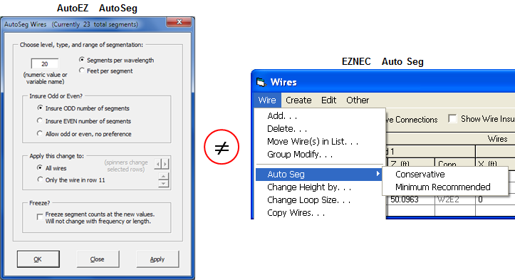
Perhaps the best way to explain the AutoEZ AutoSeg function is to show how it differs from the EZNEC Auto Seg function.
To demonstrate that last point open BYDIPOLE.ez. Use the AutoSeg button to set the segmentation to 100 segments per wavelength, odd. In the "For Information Only" columns switch back and forth between showing lengths in "ft" and "wl" (wavelengths).
- The EZNEC function offers two choices, Conservative and Minimum Recommended. Conservative results in 20 segments per wavelength. Minimum Recommended results in 10 segments per wavelength. With AutoEZ you can choose any segmentation density you desire.
- EZNEC applies the chosen segmentation to all wires of the model. With AutoEZ you can apply the change to all wires or to a subset of wires. The subset choice is set to those rows that were selected prior to clicking the AutoSeg button. You can select any column or columns from the desired rows.
You can then use a different segmentation level for other wires of the model. For example, you may wish to use a higher level for wires that carry more current and a lower level for wires that carry less current, such as radials for a vertical or guy wires for a tower.
If you use the Apply button of the dialog window rather than the OK button you can read the new total number of segments both in the dialog title and just below the "Segs" column header on the Wires sheet. That way you can adjust the segmentation level if you are trying to stay below a maximum allowed number.
- With AutoEZ you have a second choice for the method of segmentation. You can specify a physical length for each segment. This second method may be useful in cases where it is important to keep the segment junctions aligned between closely-spaced wires.
- With AutoEZ you can use a variable name such as "=A". (Or, since this is in a dialog window rather than a cell on a worksheet, just "A" without the leading "=" sign.) You can include simple operators if you wish, such as "=A/2", if you want to assign "A" segments per wavelength to some wires and half that segmentation density "A/2" to other wires. Then you can vary the value for A (or whatever variable name you used) in test case rows on the Calculate sheet to see how the Source R/X, Max Gain, Average Gain Test, and other items vary as the segmentation level is changed. More on that in the "Convergence Testing" section of this page.
Important: Note that the variable is not the "number of segments" per wire. Instead, the variable is used in a more complex formula such that each wire will have A "segments per wavelength" or A "feet per segment" as explained in the next bullet.
- By far the most important difference between EZNEC and AutoEZ is that with AutoEZ the segmentation level will automatically adjust if the length of the wire changes or if the frequency changes (which means that the length of a wavelength changes). That's because AutoEZ uses a formula to set the segmentation.
For example, if you request 20 segments per wavelength guaranteed odd AutoEZ will build a formula like this for the "number of segments" for each wire:
=ODD(WireLen / WL * 20)"ODD" is an Excel function that returns the argument (the part between the parenthesis) rounded up to the nearest odd integer. WireLen is abuilt-in AutoEZ variable that is always equal to the length of the wire (each different wire) in the current units. WL is abuilt-in AutoEZ variable that is always equal to the length of a wavelength in the current units and at the current frequency.So, for example, if a particular wire is 33.43 ft long and the current frequency is 14 MHz which means that a wavelength is 70.255 ft, the above formula would be equivalent to:
=ODD(33.43 / 70.255 * 20)If the length of the wire is changed, either by manually changing one or more XYZ coordinates or by changing the value for a variable via a test case row that results in a change to one or more XYZ coordinates, the value for WireLen will automatically change. (And remember, WireLen is unique for each wire of the model. You might think of it as many separate variables, "WireLen for wire 1", "WireLen for wire 2", etc.) If the frequency is changed, either manually or via a test case row, WL (wavelength) will automatically change. If either or both of those
or
=ODD(9.517)
or
=11built-in variables change, the segmentation may change depending on the results of the evaluation of the above formula.
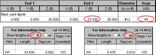
The wire is 33.43 ft long and there are 49 segments so each segment is
33.43 / 49 or 0.682 ft long. Since you requested 100 segments per wavelength each segment is also1 / 100 or 0.01 wavelengths long.Don't let the "103" in the
"Segs / wl" column fool you. That is a rounded value which is designed to let you see at a glance the approximate segmentation density for any given wire. If you temporarily deselect the "Display numbers with 3 decimal places" option you'll see (in column M) that each segment is actually 0.009711 wavelengths long (at 14 MHz). That's wavelengths per segment. The inverse of that number is segments per wavelength which equals 102.9764 which is rounded to 103 in column N.Now change the
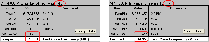
End 2 Y coordinate from 33.43 to 31.43. Notice that the number of segments automatically changes from 49 to 45. Also note that each segment is still 0.01 wavelengths long. (Actually, each segment is now 0.0099416 wavelengths long. The inverse of that number is 100.5879 which is rounded to 101 in column N.)

You can also experiment with changing the value for Freq on the Variables sheet (cell C11). Notice how the WL value changes. If you change Freq from 14 to 14.35 MHz the number of segments will change from 45 to 47 but each segment will still be (approximately) 0.01 wavelengths long, just as you requested.
Optional: There may be times when you do not want the number of segments to change. This is especially true when using the AutoEZ optimizer with multiple frequencies in the same band. In the previous illustration you saw how the number of segments changed from 45 to 47 when the frequency changed from 14 to 14.35 MHz. That means that a new model file would have to be built to pass to EZNEC for each frequency. The extra processing to do so is inconsequential for a few or even a few dozen calculations. However, when optimizing you may be doing several hundred or even several thousand calculations. In that case it is more efficient to build a single model file and pass it to EZNEC with instructions to calculate at multiple frequencies.
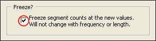
If you do not want the number of segments to change you can check the option box at the bottom of the AutoSeg dialog window. If that box is checked it is exactly as if you had manually typed in the actual number of segments that AutoSeg computes for each wire. The segment counts are "frozen" in that, being actual numbers rather than numbers set via formulas, they won't change as the frequency changes.
Convergence Testing with a Delta Loop
Open model file "Delta Loop.weq". This is a three-sided (hence Greek letter Δ) loop with the upper sides equal in length and a right angle at the apex. (Technically that makes the shape a right isosceles triangle.)
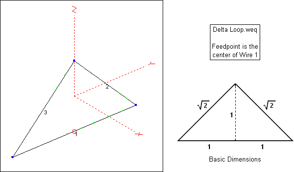
The variables for this model are initially set as follows. Note that the circumference of the loop in "basic dimensions" is
2 + 2 * SQRT(2) , so if the actual circumference is A then variable E (±Y coordinate and base to apex, "1" in basic dimensions) can be defined as shown.
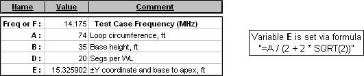
Once E has been defined the XYZ coordinates can be set via simple formulas. Wire 1 is the horizontal base wire.
The segmentation is set with AutoSeg using "=D" (or just "D") segments per wavelength, odd, so the formula for each Segs cell is
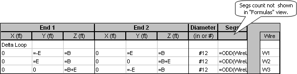
=ODD(WireLen / WL * D)On the Calculate sheet the test cases are set with D ranging from 10 to 150 segments per wavelength. Before doing the calculations select the With E/L/AGT option and click the E/L/AGT button until the column header is Avg Gain Test.
Calculate. On the Triple chart sheet the "R and X" chart looks like this.
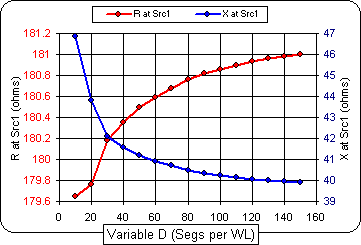
Because the left and right axes do not have the same scale it appears that both R and X vary by about the same amount as the segmentation density is increased. Closer examination shows that R (left scale) changes by only a few ohms while X (right scale) changes from roughly +j47 to +j40 ohms. It's up to you to decide what level of segmentation is adequate, making the trade-off between accuracy and processing time.
Tab to the Custom chart sheet and plot "Avg Gain Test Factor" on the Y axis and "Variable 1" (D) on the X axis. Be careful to plot "Avg Gain Test Factor" and not "Avg Gain Factor". You may wish to review the difference as explained in the Calculate Efficiency / Loss / Average Gain Test section.
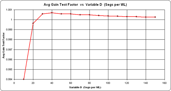
Again, pay attention to the scaling. Even at only 10 segments per wavelength the AGT value is 0.994 which is more than adequate.
AutoSeg with an LPDA
The previous two examples were a bit contrived just to illustrate how AutoSeg works. After all, it's not very likely that you would assign 100 segments per wavelength to a backyard dipole. The next two examples will show a more realistic use of the AutoSeg feature.
Open sample model "W4RNL LPDA 8504AS.ez".
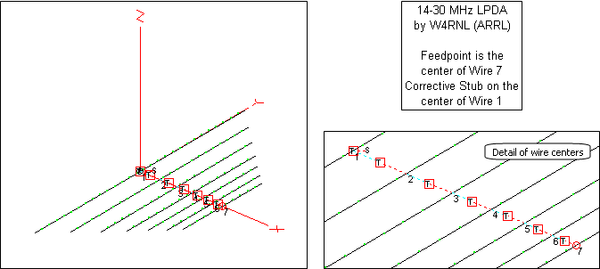
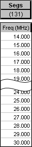
This is a design by W4RNL (SK) with tau=0.85 and sigma=0.04. It is described in detail in recent editions of The ARRL Antenna Book. The EZNEC model has a fixed number of segments (131) which is equivalent to approximately 28 segments per wavelength at 28 MHz. That's slightly above the EZNEC "conservative" guideline of 20 segments per wavelength. However, at 14 MHz the equivalence is approximately 56 segments per wavelength, well beyond the "conservative" guideline. In order to have enough segments at higher frequencies, "too many" are used at lower frequencies.
You could use AutoSeg in two different ways in this situation. First, you could assign 28 segments per wavelength. At 14 MHz the total number of segments would be 73 instead of 131 which would save a bit of processing time, although with today's computers the difference would not be very significant. (This model has 7 elements. LPDAs with more elements would show larger differences.)
Second, you could assign S segments per wavelength (or any variable of your choice) and then do a convergence test at both the low and high frequencies to help you decide just what level of segmentation density meets your needs. For example, you might set up a series of test cases as shown below on the left and then note the difference in results as shown on the right. (All 12 test cases were run at the same time. The dashed line was added for clarity in the illustration.)
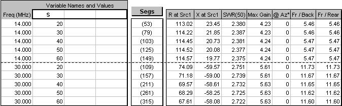
Notice that at 14 MHz the source resistance increases (113.02 to 114.57 or +1.4%) as the segmentation density goes up. At 30 MHz the source resistance decreases (74.09 to 67.61 or
Regardless of the segmentation density you feel is appropriate it's interesting to see how the currents on the wires change as the frequency changes. The elements carrying the most current progress towards the front of the array as the frequency increases. In the animation below the frequency is being swept from 14 to 30 MHz. Each "wave" on the chart represents the current in one element of the LPDA. (You can see the frequency in the lower right corner of the chart. For this illustration the original model with a fixed segment count of 131 was used.)–8.7%) as the segmentation density goes up. Subtle differences like that are easy to spot when you can quickly adjust the segmentation.
(Press Esc to stop the animation, F5 to restart.)
Cautions for the Currents Chart
When showing the currents from multiple wires it is important to remember that the AutoEZ Currents chart shows each segment in the order in which it is found in the table of currents that is produced by EZNEC. This order may not correspond to the physical position of the segment, depending on how you have defined the wires of your model.
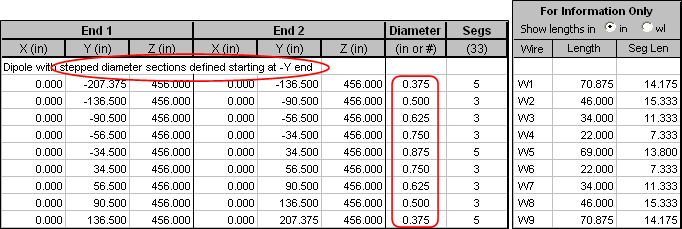
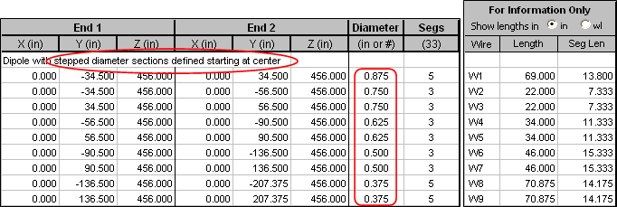
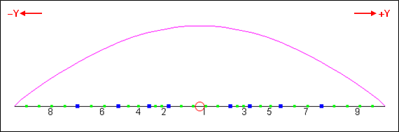
For example, here is the wire table for a 20M dipole (sample "Stepped Dipole 1.weq") built with stepped diameter wires representing telescoping aluminum tubing. The individual wires are defined in order from
-Y to +Y coordinates. Notice that the smallest diameter (0.375") wire is first, the diameters increase up to the center wire (0.875"), and then decrease back down to the smallest (0.375") again. Also,End 2 of one wire corresponds toEnd 1 of the next wire.
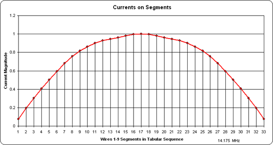
If you calculate this model and then view the currents with EZNEC you would see this.
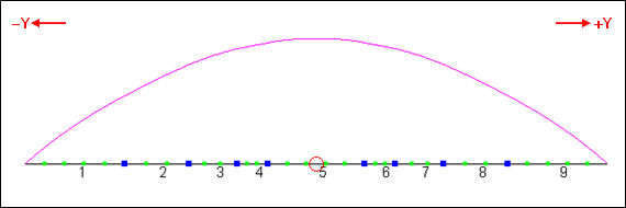
Then if you tab to the AutoEZ Currents sheet and show all wires you would see this.
So far so good. But many times you may build a model based on a "taper schedule" from a publication or web site. The taper schedule will list only the wires on one side of the element. You might then define all the "positive Y" wires first and then the "negative Y" wires, or you might define both sides for the same diameter and then move on to the next diameter as shown below (sample "Stepped Dipole 2.weq"). Notice that the largest diameter (0.875") wire is first, then both 0.750" diameter wires, then both 0.625" diameter wires, and so on.
When viewing with EZNEC the "current shape" is the same although the numbering of the individual wires in the element is different along with which wire has the source.
But on the AutoEZ Currents chart, since the wires and segments are ordered in the sequence in which they appear in the EZNEC table of currents, you would see this.
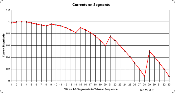
On the left are the 5 segments of wire 1, then 3 segments each of wires 2 and 3, the same for wires
4-5 and6-7 , and finally on the right the 5 segments of wire 8 and the 5 segments of wire 9. This is the order of the wires and segments in the EZNEC currents table but it is not the physical position of the segments.
Auto-Switched Sources/Stubs with a Multi-Feedpoint Pentaband Quad
The last example of using AutoSeg will be for a 5 band quad. Besides showing differences due to segmentation density this example also shows how to automatically change the location of the source for a model that has a different feedpoint for each different band of operation. And it illustrates that when you make the model more realistic by including portions of the feed system the results can change dramatically.
Open model "Pentaband Quad Square.weq".
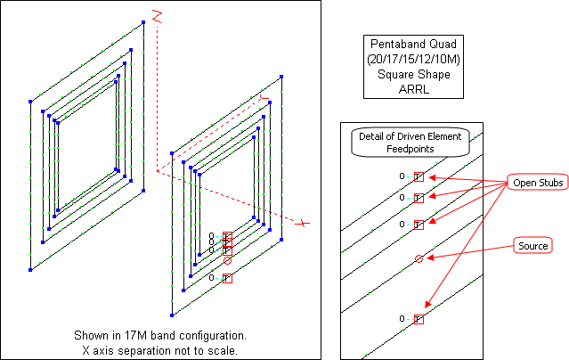
This model is described in recent editions of The ARRL Antenna Book under the heading "A Two-Element, 8-Foot Boom Pentaband Quad". It is unique in that it includes not only the antenna but also a portion of the feed system.
Each driven element loop is fed via a section of
RG-213 coax. Each coax section is cut to the same length,¾-λ at 28.4 MHz, or 17.091 ft for Belden 8267. The five sections are brought back to a switchbox located on the boom. When one section is connected to the common transmission line running back to the station (not modeled), the other four sections are left open-circuited at the switchbox. Hence the four "unused" sections act like open-circuit stubs connected to the feedpoints of the "unused" driven elements.Depending on the frequency and length, the impedance at the opposite end of an open stub will be low (almost like a short) if the electrical length is an odd multiple of λ/4, high (almost like an open) if the electrical length is a multiple of λ/2, or some impedance value in between at electrical lengths between multiples of λ/4 and λ/2. And if the "opposite end" is connected where the feedpoint would be it is like placing a load at that point. A low impedance load would be like "shorting" the unused feedpoint which is probably how most modelers treat the "unused" driven element loops. A high impedance load would be like "breaking" the loop at the unused feedpoint.
For a 17.091 ft
RG-213 open stub here are some representative impedance values of what the equivalent load would be at the unused feedpoints.
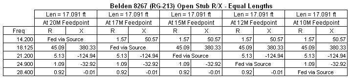
The designer of this model (unnamed) specifically chose the coax section lengths such that at 28.4 MHz the four "unused" driven element loops would be (almost) "shorted" at the feedpoints, as shown in the bottom row of the table. At other frequencies things get more complicated. For example, at 18.125 MHz (17M band) a load of 45.09+j380.33 ohms is placed at the feedpoints of all the "unused" driven element loops (20M, 15M, 12M, 10M). The results will certainly be different than if the loops were modeled with the unused feedpoints being closed connections (short circuits); that is, just a normal continuous wire with no source and no load.
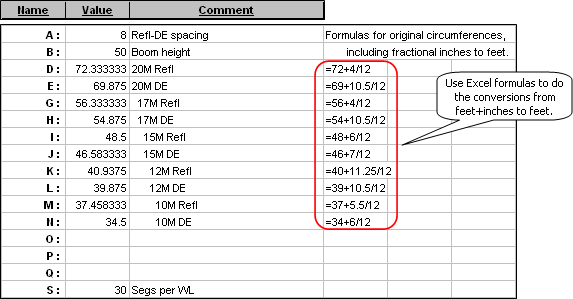
As for the actual wires of the model, the dimensions for the five reflector and five driven element loops were taken from a table in the Antenna Book. The table shows the loop circumferences in feet and inches. To build the model all dimensions had to be converted to feet and fractional feet. That's easy to do in your head if the dimension is something like
48' 6" . It's not so easy when the dimension is40' 11¼" .Here's a tip you may find useful in situations like this. Rather than use your pocket calculator to do the inches to feet conversion, just type a formula in the scratchpad area of the Variables sheet. For example, to convert
40' 11¼" to feet and fractional feet type:=40+11.25/12When you press Enter Excel will show the equivalent value in feet. Then you can "Copy - Paste Special - Values" that result over to the "Value" column for the given variable name.
With variables for the loop circumferences defined it's straightforward to create the formulas for the XYZ coordinates. For example, the 20M reflector (wires
1-4 ) and driven element (wires5-8 ) loops are defined like this. Extensive use of the "W#E#" type shortcut to define the first loop, then Copy/Paste (to duplicate 4 rows) and Edit/Replace (to change variable names) makes the task a lot less daunting than it seems.
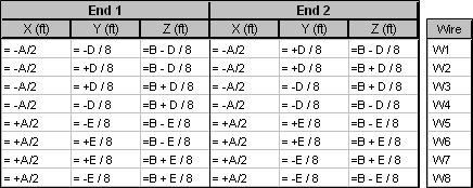
Note that the unary operator "+" (such as "+A/2") is not required. It is used here merely to make it more obvious which coordinates are "+X" axis vs
"-X" axis and "+Y" axis vs"-Y" axis.An alternative method to create the wires of the model would be to use the AutoEZ Create Wires - Loop function.
To model the sources and transmission line stubs the AutoEZ feature of "marking out" insertion objects is used, with the presence or absence of the "mark" being determined by a formula based on the test case frequency. For example, when automatically configured for the 17M band the Sources table looks like this.
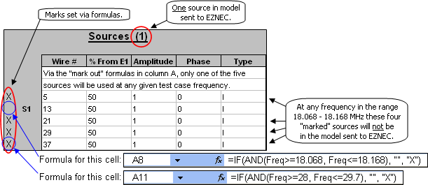
The column A "mark" formulas used for the five rows are, respectively:
=IF(AND(Freq>=14, Freq<=14.35), "", "X")To understand how this works let's look at the formula for the second row (Wire 13 / 50%). The syntax for the Excel IF function is
=IF(AND(Freq>=18.068, Freq<=18.168), "", "X")
=IF(AND(Freq>=21, Freq<=21.45), "", "X")
=IF(AND(Freq>=24.89, Freq<=24.99), "", "X")
=IF(AND(Freq>=28, Freq<=29.7), "", "X")IF(logical_test, [value_if_true], [value_if_false])and the "logical_test" can be a compound test using the Excel AND function. The syntax for the AND function isAND(test1, test2, test3 ...)For the second row, the compound "IF" condition [the AND(Freq>=18.068, Freq<=18.168) part of the formula] will be true at any frequency in the 17M band (18.068 to 18.168 MHz), hence the mark will be a null string ["", no space between the two quote marks] which is the same as no mark. At the same time, the "IF" condition will be false for all the other rows so those sources will be "marked out" [with "X"] and not included in the model sent to EZNEC. At other test case frequencies a different source table row will be used ("unmarked") depending on the frequency.It is not necessary that the frequency ranges used in the "IF" functions be exact band edges. For example, for the 20M band you might use 13 to 15.35 MHz instead of 14 to 14.35. That would allow you to run frequency sweeps outside the band. Just make sure there is no overlap in the frequency ranges so that your EZNEC model does not end up having two sources instead of just one.
It is also not necessary that the "mark" formulas be in ascending frequency order. It all depends on the order of the rows in the Sources table. If you have defined the first source as being for the 10M band then the corresponding first "mark" formula would be for the frequencies of that band.
The transmission line stubs are defined in a similar (but not exactly the same) manner. When automatically configured for the 17M band the Transmission Lines table looks like this.
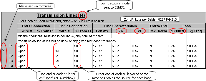
For the transmission lines the "mark formulas" have the opposite logic.
=IF(AND(Freq>=14, Freq<=14.35), "X", "")Here the open-circuit stub connected to the 17M feedpoint (Wire 13 / 50%) is "marked out" for any test case frequency from 18.068 to 18.168 MHz since that is where the source will be placed. Stubs connected to all the other driven loop feedpoints are "unmarked" and hence will be included in the model sent to EZNEC. It doesn't matter which end of the transmission line you define to be "Open".
=IF(AND(Freq>=18.068, Freq<=18.168), "X", "")
=IF(AND(Freq>=21, Freq<=21.45), "X", "")
=IF(AND(Freq>=24.89, Freq<=24.99), "X", "")
=IF(AND(Freq>=28, Freq<=29.7), "X", "")If you find the marked/unmarked concept confusing just tab to the Variables sheet and manually change the Test Case Frequency (Freq, cell C11) to a new value in a different band. Then return to the Insr Objs sheet. You'll see that a different row in the Sources table is now "live", that is, not marked and will be included in the model sent to EZNEC. You'll also see that a different row in the Transmission Lines table (corresponding to the source that is now live) is now "marked", that is, will not be included in the model sent to EZNEC.
In effect, for any given band one of the stubs "disappears" and the source is placed directly at the appropriate driven element feedpoint. That is done so you can get an impedance reading at the feedpoint. Note that the model does not include the main transmission line back to the station.
Defining the sources and transmission line stubs in this manner means you don't have to remember to manually switch the source and stub placement when changing test case frequencies. With the "multi-band, automatic-configuring" model now complete it's time to run some test cases to see what differences show up when using different segmentation density levels. The example below compares 30 segments per wavelength to 60 segments per wavelength at mid-band frequencies for all 5 bands. You'll need EZNEC+ or EZNEC Pro to duplicate this exact scenario. At 28.4 MHz with 60 segments per wavelength the total number of segments is 912, above the EZNEC Standard limit of 500. (Again, all test cases were run at the same time and the dashed line was added just for clarity in the illustration.)
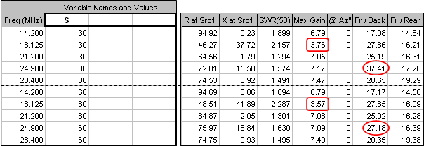
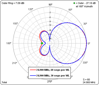
Results are similar for the two different segmentation density levels except for the
ratio at 24.9 MHz (12M band), 37.41 dB at 30 segments per wavelength vs 27.18 dB at 60 segments per wavelength. A look at the polar chart shows that the deep null at 180° when using 30 segments per wavelength has "filled in" when using 60 segments per wavelength.
It's also interesting to note that the
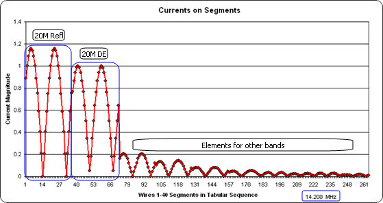
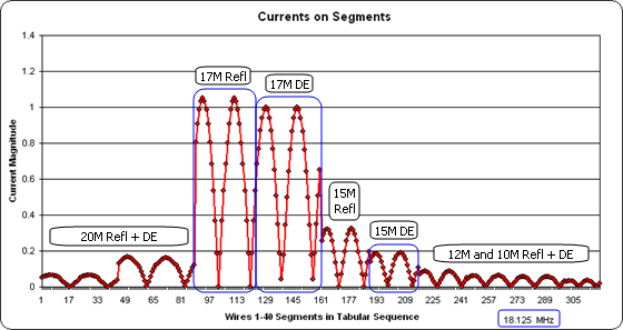
is roughly 7 dBi (6.79 to 7.49) for all bands except 17M where it drops to less than 4 dBi (3.76 or 3.57). The Currents chart gives a clue as to why that is. First let's look at the currents at 14.2 MHz (20M band). Note that the magnitudes of the currents in the elements for the "other" bands are well below those for the 20M reflector and driven element. That is, the two 20M elements seem to be well isolated from the other elements.
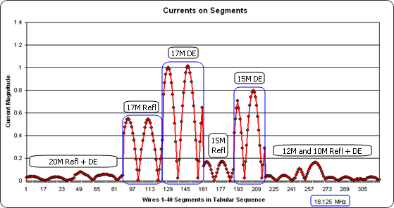
But for the 17M band things are not so clean. The 17M reflector current is much lower than it should be and the 15M driven element has a substantial amount of induced current. Remember, at 18.125 MHz the 15M driven element is not being fed with a source. Instead, it has 45.09+j380.33 ohms placed where the feedpoint would be. So instead of being a continuous wire closed loop the 15M driven element is much closer to being an open loop, with a related change in the resonance. In effect the 15M driven element loop has "robbed" induced current from the 17M reflector loop, thus lowering the gain on 17M.
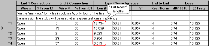
In the model as described in the Antenna Book all five stubs were cut to the same length,
¾-λ at 28.4 MHz or 17.091 ft. But what if they had been cut to the "just reach" length, from the switchbox to the feedpoint for any given driven element loop. For example, if we assume that the switchbox is located at the center of the 8 ft boom, for the 20M loop it would be 4 ft from the box to the spreader hub and then "E/8" or 8.734 ft down to the feedpoint for a total length of 12.734 ft. For the 10M driven element loop the "just reach" length would be "4+N/8" or 8.313 ft. Lines to the other feedpoints would fall somewhere in between. When configured for the 17M band the Transmission Lines table now looks like this.
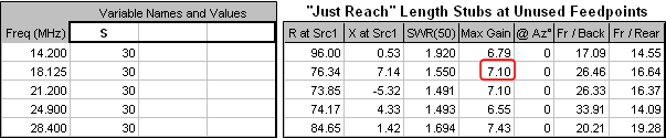
Did this change in stub lengths make any difference in the Max Gain on 17M? You bet it did. At 30 segments per wavelength the Max Gain is now 7.10 dBi compared to 3.76 with the "equal length" stubs.
And the Currents chart shows that at 18.125 MHz the 15M driven element is no longer "robbing" induced current from the 17M reflector.
The lesson in all this seems to be that if you have a multi-band antenna with separate feedpoints all connected to a common switchbox, the "unused" feedlines at any given frequency will act like open stubs (or perhaps like shorted stubs if the switchbox "shorts out" unused lines). And if those stubs happen to present a high impedance at the "unused" feedpoints it will definitely affect the performance of the model.
As you've seen from the above example it's relatively easy to include the stubs in your model and make them, and the source, "frequency agile" so you don't have to remember which wire gets what when changing bands. Your modeling results will then be one step closer to representing reality and you can do "what if" experiments to determine optimum stub lengths.