An Excel (XL) workbook to calculate antenna gain/temperature ratio (G/Ta), average gain, directivity, and other metrics by using 3D pattern data from EZNEC, AutoEZ, 4nec2,A.M. , MMANA-GAL, or HFTA.
Contents
- Creating 3D radiation pattern data files
- Calculating G/Ta and other 3D metrics
- Applying the KF2YN correction
- Applying the Average Gain Test correction
- Hints
- Theory of operation
- Showing 3D plots and Saving 2D Slices
- References
- Download
- Acknowledgments
The first step in using XLGTa is to create a file containing 3D radiation pattern data in OpenPF (.pf3) binary format, comma-separated values (.csv) text format, or VOACAP type 13 format (.13). You can utilize any of several different programs.
Creating 3D radiation pattern data filesNo matter which program is used, if the ground type is not Free Space then no temperature calculations will be done. Only general purpose metrics such as max gain, average gain, directivity, and several others will be calculated.
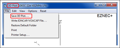
Set the Plot Type to 3D and choose a Step Size, usually 1 degree but may be any value which divides into 90 evenly such as 2 or 3 or 5 degrees. Click the FF Plot button. From the 3D Plot window click File > Save 3D Plot. In the "Save Trace" dialog that will appear enter a descriptive file name, something that will allow you to associate the pf3 file with a particular antenna model file. The folder for the pf3 file need not be the same folder that contains the XLGTa workbook nor the same folder where the EZNEC model file (.ez) is located.
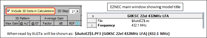
On the Calculate tab enable the "Include 3D Data in Calculations" option and set the desired 3D step size. For each calculated row (each test case) a file named $AutoEZ$n.PF3, where "n" is the test case number, will be written to the AutoEZ home folder. When the XLGTa workbook reads such files the text from cell B10 on the AutoEZ Wires sheet tab, which is used to set the EZNEC "Description Title" (top of the EZNEC main window), will be shown along with the actual file name of the pf3 file.
The $AutoEZ$n.PF3 file may be copied to a different folder and given a different file name if desired.
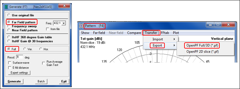
Click Calculate > NEC output-data. In the Generate dialog choose Far Field pattern and set the desired Frequency. Choose option Full and set Resol[ution] (Step Size). Click Generate. When the calculation finishes, on the Pattern window click Transfer > Export > OpenPF Full/3D. In the "Save File (As)" dialog that will appear the default file name will have the step size appended at the end. The default save location will be the 4nec2 \plot folder but you may navigate to any other folder of your choice.
/font
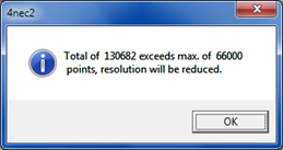
If you see an error message with the words "Total of xxx exceeds max of yyy points" you must change one of the 4nec2 options. On the main 4nec2 window click Settings > Memory usage >
Max-nr field-points . For 3D patterns with a 1 degree step size enter a value of 130682 or greater in the small 4nec2 prompt. Exit and restart 4nec2.
• With A.M. (Antenna Model by Teri Software):
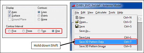
Click Calculate > 3D Radiation Pattern. In the 3D window make sure the Contour Interval (Step Size) is set as desired. Click File then hold down the Shift key and click Save 3D Pattern Data. In the "Save As OpenPF File" dialog that will appear you may modify the file name and/or navigate to a different folder if desired.
If you do not hold down Shift before choosing Save 3D Pattern Data the pf3 file will be automatically written to the last-used "archived generated output products" folder, overwriting any existing file with the same name. For more information concerning the current location of the "archive" folder see topic "Where's My Files?" in the A.M. Help.
The programs mentioned above all save the 3D data in the OpenPF (pf3) binary format. MMANA saves 3D data in comma-separated values (csv) text format. For this format the XLGTa workbook will assist you by providing the correct parameters for MMANA. In the XLGTa workbook choose the "MMANA csv" Source Type option. Enter your desired step size and free space (True/False) choices. Be sure to make entries only in the yellow-shaded cells.
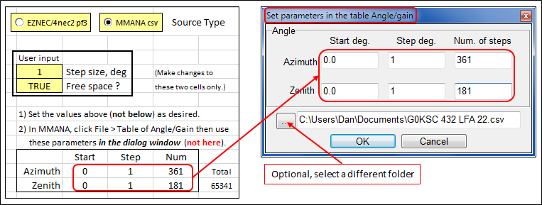
In MMANA, open a model and set your desired "Ground" and "Material" (wire loss) choices on the Calculate tab. Click Start to do a calculation. Click File > Table of Angle/Gain. In the MMANA dialog window change the "Step deg" and "Num of steps" entries to match exactly what is shown by XLGTa. If desired use the small "..." button on the MMANA dialog to navigate to a different folder and enter a different file name. Note that you must still click OK on the MMANA dialog window to create the csv file. Optionally you can just type in a new folder and/or file name in the MMANA dialog window and then click OK.
A few things to keep in mind when using MMANA:
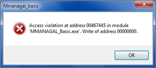
- After creating a csv file, if you subsequently make any changes to the model such as changing the Material (wire loss) setting, you must click Start again to do another calculation. If you click File > Table of Angle/Gain after making a change but without doing a recalculate, when you attempt to create the csv file you'll get an "Access violation" error message. Just close the message window and click Start to do a calculation.
- The csv files produced by MMANA will always use a period as a decimal separator and a comma as a field delimiter regardless of your regional settings. If your regional settings have the decimal separator as a comma and the field delimiter as a semicolon then the MMANA csv files cannot be opened (correctly) using the normal Excel user interface. However, you can always inspect the files using Notepad.
- Use what is shown by XLGTa as a guide to set the MMANA dialog fields. Do not change the XLGTa cells directly, that's an easy mistake to make. (And if you do no harm will be done, you'll just get a warning.)
- The OpenPF (pf3) files mentioned earlier contain frequency information which is appended to the file name for display by XLGTa. The MMANA csv files do not contain any frequency information. You may wish to manually modify the default file name to include the current frequency.
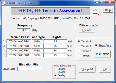
The High Frequency Terrain Assessment (HFTA) program by Dean Straw, N6BV, when used in conjunction with the MakeType13 or HFTASweep utility programs, can create a special "omni-directional" VOACAP type 13 3D pattern file. Type 13 files are typically used with VOACAP and similar propagation prediction programs.
More conventional (not omni-directional) type 13 files can be produced by EZNEC and 4nec2. With EZNEC, set the Plot Type to 3D, set the Step Size to 1 degree (only), and make sure the Ground Type is not Free Space. Click the FF Plot button. From the 3D Plot window click File > Write IONCAP/VOACAP File.
With 4nec2, assuming the ItsHF package has been installed, click Calculate > NEC output-data. In the Generate dialog choose ItsHF 360 degree Gain Table. Set the desired Frequency and the various options for ItsHF. Click Generate. A file with extension *.n13 will be created in the C:\itshfbc\antennas\4nec2 folder.
In addition, several years ago L. B. Cebik created dozens of conventional (not omni-directional) type 13 files using EZNEC. See VOACAP Type-13 Files for Amateur Band Antennas and Sample Azimuth Patterns. You can download any of these files and plot them as desired.
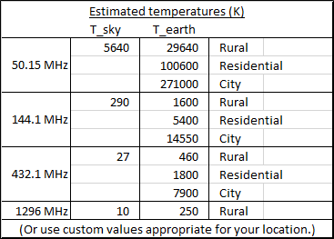
After a 3D pattern data file has been created the next step is to set the T_sky and T_earth temperatures. A listing of suggested temperatures is included on the first workbook sheet. (If the 3D pattern data is not for Free Space the T_sky and T_earth settings are ignored.)
Calculating G/Ta and other 3D metrics
With T_sky and T_earth set as desired, click the
Read ... button to read a 3D data file. You can follow the progress of the calculations by noting the changing status bar text in the lower-left corner of the Excel window, where READY is normally displayed. You'll see:Opening pf3 [or csv] file ...If the step size of the current file differs from that of the previous file you'll also see:
Copying from pf3 [or csv] file ...
Gain/Temperature ...
Calculating rows ...Filling down more rows ...Additional rows at the bottom of the first sheet are automatically added or deleted as necessary to accommodate the number of data points in the file.
or
Deleting unused rows ...When the calculations are complete several general purpose metrics are shown including 3D Maximum Gain, Average Gain, Directivity, Rear Hemisphere Average Gain, and Rear Hemisphere Mean Sidelobe Level.
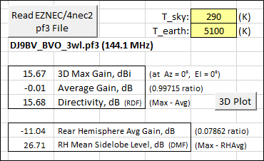
Note that whereas Directivity equals (in dB terms) Maximum Gain minus the Average Gain over all directions, Rear Hemisphere [RH] Mean Sidelobe Level [MSL] equals Maximum Gain minus only the Rear Hemisphere Average Gain. In this context "Rear" means the hemisphere of the 3D radiation pattern that is opposite the main forward lobe. For more information on these and other terms see this IEEE document, this Cisco document, and this ARRL presentation.
In amateur radio literature Directivity is also known as RDF (per W8JI) and RH MSL is also known as DMF (per ON4UN). See chapter 7, sections 1.8, 1.9, 1.10 in Low-Band DXing 4th or 5th editions by ON4UN. If the 3D pattern data is not for Free Space then "Rear Hemisphere" is actually "Rear Quadrisphere" or "Rear Half-Hemisphere".
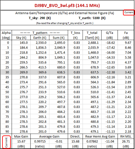
Using the entered T_sky/T_earth settings the various antenna temperature results will be shown in the "Current" table. The general purpose metrics are duplicated at the bottom of the table. (If the 3D pattern data is not for Free Space the general purpose metrics described above will be calculated but no temperature calculations will be done.)
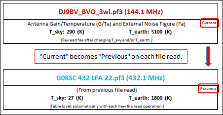
On each file read operation the former entries in the "Current" table will be automatically transferred to the "Previous" table. That way you can easily compare the response for two different antennas or for the same antenna with different levels of segmentation density in the model.
You can also view a chart that shows either the anstenna gain/temperature ratio (G/Ta) or the external noise figure (Fa) for both the "Current" and "Previous" files. External noise figure Fa is calculated as 10*Log10(T_pattern/290). For more information see Section 2 of this ITU document. (Note that some images on this web page show Fa as calculated using a previous formula.)
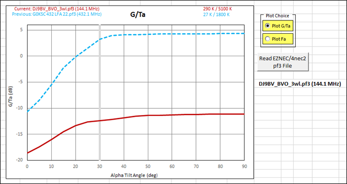
In the image above note that the antennas are for two different bands with two different settings for T_sky/T_earth. That was done merely for illustration. Also note that if the KF2YN correction option is enabled (see next section) a third trace line will be shown on the chart.
The secondary
Read ... button near the chart makes it easy to quickly compare multiple antennas as long as the T_sky/T_earth temperatures do not need to be changed. Or just scroll over to the primaryRead ... button if you do need to change T_sky/T_earth for the next file to be read.In order to calculate T_loss and T_total [Tant] an assumption is made that if the antenna has no wire loss the Average Gain ratio will be exactly 1. With loss included, such as Aluminum instead of Zero for wire loss, the Average Gain should always be less than 1. If the calculated Average Gain is greater than 1 by a non-trivial amount
Applying the KF2YN correction(>= 1.00050) the ratio will be displayed with a red font and a red warning will be shown. The threshold of 1.00050 means that EZNEC would show "Average Gain = 1.001" or greater and 4nec2 would show "Radiat[ion]-eff[iciency] 100.1%" or greater.For some antenna configurations, especially Yagis with loop or folded dipole driven elements, various NEC limitations make it difficult or impossible to achieve an Average Gain of exactly 1 for a no-loss model. To address that situation Brian Cake, KF2YN, developed an algorithm which can correct the calculated antenna gain and temperatures given the "No Loss" and "With Loss" data for an otherwise identical antenna model. The KF2YN algorithm can be used when the Average Gain is less than 1 or greater than 1.
Taking advantage of the presence of the "Current" and "Previous" tables, the KF2YN correction algorithm has been incorporated into the XLGTa tool. No special action is needed other than to first read a "With Loss" file; typically a file generated with wire loss set to Aluminum. Then read a "No Loss" file for the same antenna; a file generated with wire loss set to Zero. The "No Loss" calculated results will then be in the "Current" table and the "With Loss" results will have been automatically transferred to the "Previous" table.
Using information from both tables, the "Corrected" data will be shown in a third table. Here is an example with the middle portion of each table removed for brevity.
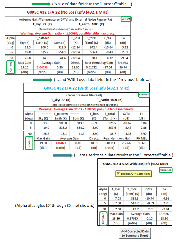
When using the KF2YN correction it is important that both the "With Loss" and "No Loss" data files are generated at the same segmentation density since a change in the segmentation will usually lead to a change in the frequency response. The "With Loss" and "No Loss" files should be identical with the sole exception of wire loss.
If you inadvertently reverse the order of reading the "With Loss" file (should be read first) and the "No Loss" file (should be read second) you'll see a different red warning at the top of the "Corrected" table.
If the "Current" and "Previous" tables are not for the same antenna you can just ignore the "Corrected" table since in that case the KF2YN algorithm does not apply. Optionally you can disable the KF2YN corrections using the checkbox; the entire "Corrected" table will then appear empty.
If you want to save the corrected data, perhaps for comparison with other antennas, use the
Add ... button located just below the "Corrected" table. For convenience there is a secondaryAdd ... button located just to the right of the table. Either button may be used. Also for convenience, instructions for use of the KF2YN correction are shown in column AQ of the XLGTa workbook just to the right of the table.The KF2YN correction algorithm has been implemented in an online JavaScript calculator developed by Hartmut Kluever, DG7YBN. You can use that online calculator to verify the XLGTa calculations if desired. For example, using data from the illustration above:
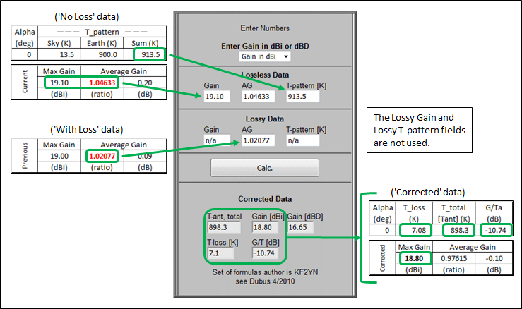
Note that showing the Average Gain ratio to five decimal places really cannot be justified given the precision of the dBi values in the data files. The fifth decimal is shown only to allow an exact comparison to the DG7YBN online calculator.
If Average Gain is calculated for a
Applying the Average Gain Test correctionno-loss model the resulting AG value is sometimes called the Average Gain Test (AGT) value. The AGT value can be used to correct the gain of theno-loss model. From section "Average Gain" in the EZNEC Help:When the Average Gain is one (with no loss present), the program is producing correct results. If it deviates significantly from this value, results are in error, and [the model] should be altered if possible. Every effort should be made to correct the problem. ... If it's not possible to reduce the Average Gain to nearly unity (zero dB), the gain can be corrected with fair accuracy by subtracting the Average Gain in dB from the reported field strength in dBi.If the gain has been corrected as described above then it is also reasonable to assume that (for ano-loss model) T_loss can be set to 0 K and T_total [Tant] can be set equal to (Sum) T_pattern. And when that is done new values for G/Ta and Fa can be calculated.As it turns out the KF2YN algorithm can also do a "pseudo-AGT" correction. Rather than reading a "With Loss" data file followed by a "No Loss" file, just read the "No Loss" file twice in a row. In the image below notice that the corrected Max Gain (18.90 dBi) is equal to the uncorrected Max Gain (19.10 dBi) minus the uncorrected Average Gain (0.20 dB). Also notice that the corrected T_loss is 0 K and the corrected T_total [Tant] is equal to the uncorrected (Sum) T_pattern for all alpha tilt angles.
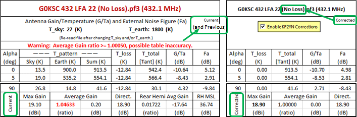
Note that the above calculations are valid only if both the "Current" and "Previous" tables contains data for a
no-loss model. There is nothing in the 3D pattern files to indicate whether the data is for a "with loss" or "no loss" model so it is up to the user to decide if the "Average Gain Test (per KF2YN) correction" calculations are applicable or not.The
Add ... button can be used to save the corrected results to the Summary sheet just as before. So if you were to read a "With Loss" file followed by a "No Loss" file, click theAdd ... button, read the same "No Loss" file again, and click theAdd ... button again, you would have a record of the "KF2YN corrected With Loss" results and the "AGT corrected No Loss" results. In the example below, rows 9 and 11.
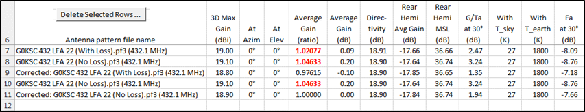
If you are not interested in the uncorrected results you can delete entire rows. In the example above, rows 7, 8, and 10. Or, just copy rows 9 and 11 to a different workbook.
For reference: L.B. Cebik has written extensively on Average Gain and the Average Gain Test here, here, and here. He has also written on the related subject of Convergence testing here and here.
Here are a few tricks which may not be immediately obvious.
Hints
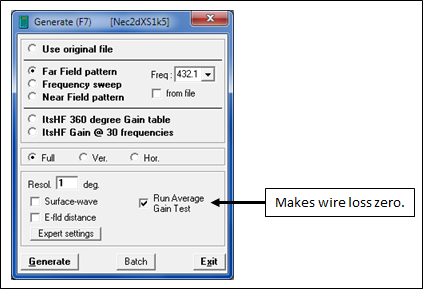
When using 4nec2 an easy way to temporarily make the wire loss zero is to enable the "Run Average Gain Test" option in the Generate dialog. That may be more convenient than removing wire loss via one of the NEC editors. Don't forget to clear the checkmark for future calculations.
On the EZNEC Wires window you can use Wire > Auto Seg > Conservative to set the segmentation density for all wires to approximately 20 segments per wavelength at the current frequency.
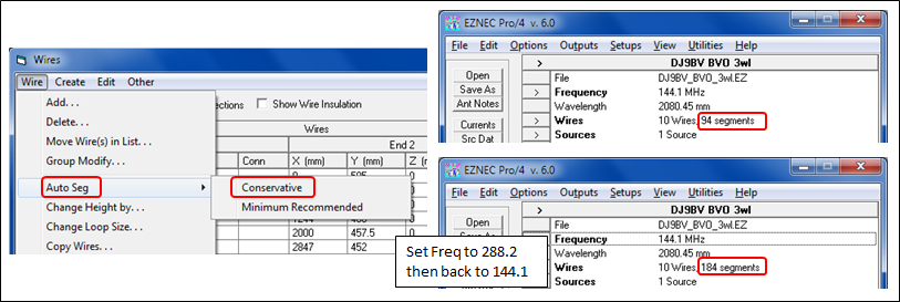
If you temporarily double the frequency, do an Auto Seg, then set the frequency back to the original value you can change the segmentation density to 40 segments per wavelength without having to manually enter a new segment count for each wire. For even higher segmentation density just use a higher temporary frequency.
With AutoEZ you can automate that process.
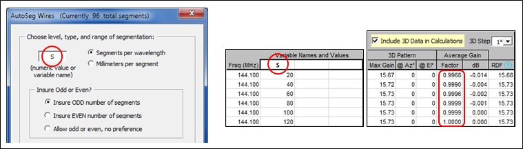
On the Wires tab click the AutoSeg button and assign S segments per wavelength (or any other variable name of your choice). Then on the Calculate tab set up a "variable sweep" on S, all at the same frequency. Enable the "Include 3D Data in Calculations" option and you can see how the Average Gain changes as the segmentation density changes.
Suppose you want to capture an image of one of the tables for documentation. Start by selecting (dragging through with the left mouse button held down) all cells in the desired table. For example, to capture the "Current" table select cells T1 through AA29. With those cells selected what you do next depends on which version of Excel you are using.
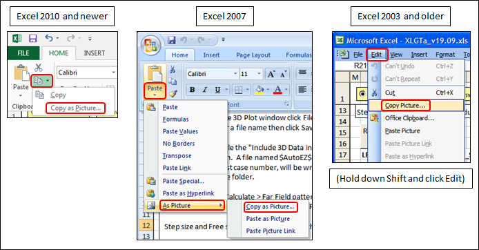
In all cases you will then see a "Copy Picture" dialog.
- With Excel 2010 and newer: In the Home tab of the ribbon, in the Clipboard group, click the arrow next to the Copy icon and select Copy as Picture.
- With Excel 2007: In the Home tab of the ribbon, in the Clipboard group, click the arrow under the Paste button, select As Picture then Copy as Picture. Why "Copy as Picture" is under the "Paste" button is something known only to Microsoft.
- With Excel 2003 and older: Hold down the Shift key and click Edit on the menu bar, then select Copy Picture.
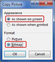
Select options "As shown on screen" and "Bitmap" then click OK. You can then paste the bitmap image into Word, PowerPoint, MS Paint, or any other application that accepts bitmap images.
You can use this same technique to capture an image of the chart. Click on the chart border to select it instead of a range of cells, then follow the steps above. After you have made the copy press Esc or click on any cell; either way will "de-select" the chart.
To see the exact value of G/Ta or Fa on the chart for any alpha tilt angle just point to one of the chart traces with your mouse. The value for the closest point will appear in a small "chart tips" window. For example, to see the G/Ta value at 30° tilt angle:
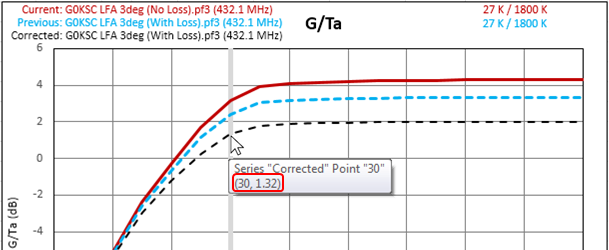
With Excel 2007 only you must first click on the chart border before pointing to a trace line. With all other versions of Excel that is not necessary.
When you scroll right to see the "Corrected" table or to view the chart you may find that when you scroll back to the left you are "over-shooting" your desired left column. If that is the case you can hide columns A:K by using the button located at the approximate position of cell R38.
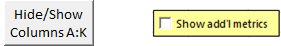
With columns A:K hidden you can scroll "all the way left" and the left-most column will be column M.
If you are wondering what happened to column L just tab to the "Summary of Metrics" sheet and enable the yellow checkbox. That will show two additional sheet tabs along with column L on the first sheet.
The tables occupy 29 rows and the top row is double height. If you are working with a limited screen size and you have a newer version of Excel you may wish to collapse the ribbon in order to gain more viewing area. You can do that as follows:
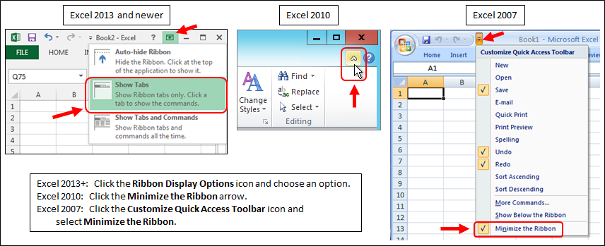
For detailed instructions see Show or hide the ribbon in Office.
Calculation of the various antenna temperatures and the G/Ta ratio is based entirely on the work of F5FOD and DG7YBN. They have documented their work extensively at Antenna G/T Calculating Software by F5FOD with DG7YBN and in Dubus magazine issues #1 through #4, 2017. Their explanations are detailed and complete so there is no need to repeat any of that here. The XLGTa macro code duplicates almost exactly the code found in the AGTC_lite and AGTC_2lite family of programs.
Theory of operationHowever, there is one very minor difference which may show up as a small discrepancy in the results when using exactly the same 3D radiation pattern data. In other words, when the FFTab .txt dBi values for AGTC_2lite and the OpenPF .pf3 dBi values for XLGTa are identical.
In order to do the calculations it is necessary to divide the 3D radiation sphere into small "patches" of surface area. These surface area patches are measured in units of steradians. The sum of all the surface area patch steradian values should equal exactly 4π, the surface area of a sphere having a radius of 1 unit.
The AGTC series of programs uses the "Differential Solid Angle" formula as shown in this extract from Geometry of Radiation:
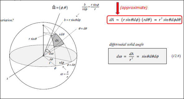
Notice that the formula for the patch area dA uses the "almost equal to" (≈) symbol. The formula is exact only if the step size of both theta (θ) and phi (φ) is infinitely small. Since the AGTC programs use a step size of 1 degree, which is indeed small but not infinitely small, the sum of all the patch areas is not quite 4π for the full sphere. Instead, the sum is 99.9975% of 4π.
Jean-Pierre, F5FOD, mentions this small difference on page 21 of Dubus #1, 2017:
Why is that tiny delta? Because unlike dθ, dφ the Δθ, Δφ [the 1 degree step sizes of θ and φ] are not infinitesimal quantities. Hence the trapeziums ... do not exactly follow the red curve. Thus we miss a small percentage of the surfaces.On the other hand, XLGTa uses the "Finite Solid Angle" formula for the size of the surface area patches.
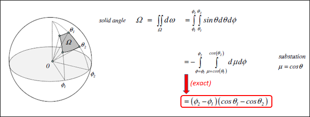
This is the same technique that is used in the Fortran code of the
NEC-2 andNEC-4 engines to calculate average gain. Using this alternative method to calculate the size of each surface area patch means that the sum will be exactly 4π, even when using larger step sizes such as 2, 3, or 5 degrees.So how does this incredibly small difference show up in the results? Here is a comparison for a 6m Yagi model developed by KF6A.
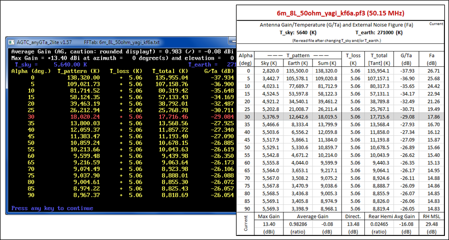
When the small discrepancy in surface area is combined with the relatively large T_sky/T_earth temperatures typical for 50 MHz the difference between using the "Differential Solid Angle" formula versus the "Finite Solid Angle" formula is just barely noticeable. Of course this makes no practical difference. It is mentioned here merely to address the potential question of "Why don't the two programs produce exactly the same results?"
If you have generated several (or several dozen) *.pf3, *.csv, or *.13 3D pattern files you can refresh your memory as to what the pattern looks like without having to recalculate the original model. Or you can create the model and pattern with one program and then use a different program to see a 3D plot, since each of the 3D viewers described below has its own set of features.
Showing 3D plots and Saving 2D SlicesTo use the 3D Plot button requires that you first use the Browse button to set the path (cell N27) to one of five supported viewers:
If you would like to use multiple viewers you can copy/paste cell N27 to a cell a few rows down. Then set the path to a different viewer and copy/paste that as well. You might end up with something like this.
- EZNEC v. 5.0 or v. 6.0 or v. 7.0 using TraceView mode. The EZNEC Pro+ v. 7.0 program is now free.
- 4nec2 using the Viewer (F9) window. Be sure you have the most recent 5.8.17 4nec2 release.
- LBDXView from the ON4UN Low-Band DXing 5th edition CD.
- NECPlotG from the Lawrence Livermore National Laboratory (LLNL) NEC-4.2 CD.
- NEC5GI from the Lawrence Livermore National Laboratory (LLNL) NEC-5 download package.
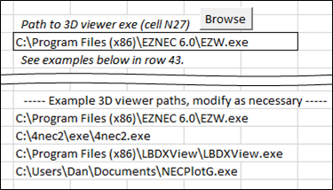
Then you can copy/paste back into cell N27 your current choice. Whatever path is in cell N27 when you click the 3D Plot button is the viewer that will be used.
All of the above programs have extensive Help files so detailed instructions for use will not be given here. After setting the path, when you click 3D Plot what happens next will depend on which viewer you have chosen.
• With EZNEC:Using the current contents of columns A through E in the XLGTa workbook a "$Temp$.pf3" file will be generated, EZNEC will be started if not running already, TraceView mode will be selected, and the EZNEC 3D Plot window will be displayed. If desired you can then also show the 2D Plot window.
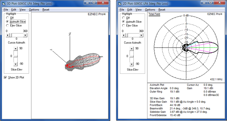
A Reset EZNEC button will appear below the XLGTa 3D Plot button. When you are done viewing 3D plots you can use the Reset button to put EZNEC back into normal mode operation. Or you can just close the EZNEC window.
• With 4nec2:If 4nec2 is running already it will be closed and restarted. A "$Temp$.out" file will be generated by XLGTa. This is an abbreviated form of the output file from a NEC engine. The file contains radiation pattern data but no wire, segment, or current data. It will be opened by 4nec2 and the Viewer (F9) window will show the 3D pattern. The Pattern (F4) window will also be shown.
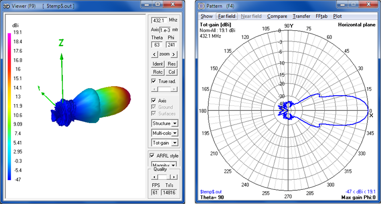
A Reset 4nec2 button will appear below the XLGTa 3D Plot button. When you are done viewing 3D plots you can use the Reset button to put 4nec2 back into normal mode operation. Note that if you close 4nec2 without using the Reset button, the next time you manually start 4nec2 you will see a standard Open dialog window with the "Files of type" drop-down set to "Nec output files (*.out)". To open a normal *.nec input file you will have to change the file type selection to "Nec input files (*.nec)". If you use the Reset button the file type selection will be changed back to *.nec for you.
• With LBDXView:Before using LBDXView as a viewer from XLGTa you must first make sure that LBDXView can display 3D patterns. Start LBDXView manually and look for a "3D" tab. If you see only tabs for Pattern, Graph, and Data Grid it means you are missing certain DirectX components. Click Help > Check Direct3D Status and you will probably see an error message. You can download the missing components from the Microsoft DirectX End-User Runtime Web Installer site.
After you have confirmed the presence of the LBDXView 3D tab you can close the program. It will be started automatically by XLGTa.
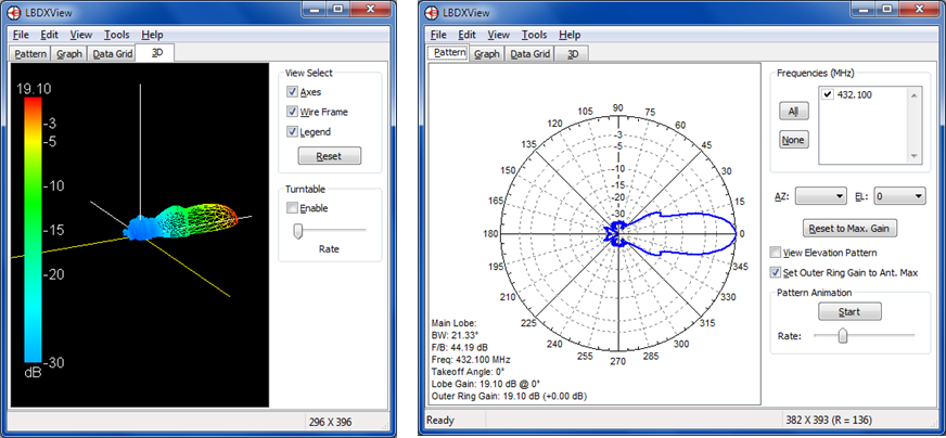
Note that LBDXView is designed to display patterns over ground, not free space. So if the XLGTa workbook currently contains a Free Space pattern only the "top half" of the pattern will be sent to LBDXView in the form of a "$Temp$.pf3" file. If you roll the 3D pattern around you'll see that it's "empty" on the bottom.
If you try to open a Free Space pf3 file directly with LBDXView the program will terminate abnormally.
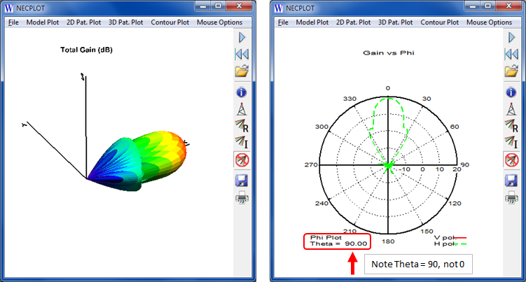
• With NECPlotG or NEC5GI:The NECPlotG and NEC5GI programs show the 3D and 2D patterns with a linear dB scale, not the usual ARRL modified log scale. With linear scaling (at the default range) the minor lobes of the pattern appear very much reduced.
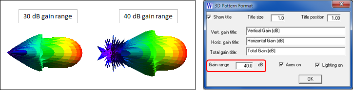
The NECPlotG/NEC5GI default linear range for the 3D plot is 30 dB. If you want to show the minor lobes of the pattern that are more than 30 dB below the max gain you can click 3D Pat Plot > Format and then in the small dialog window that will appear change the Gain range from 30 to 40 dB.
If you have 4nec2 installed you can compare linear scaling with ARRL scaling by changing the "ARRL style" checkbox on the Viewer (F9) window. On the Pattern (F4) window you can click Far Field >
ARRL-style scale or press keyboard "L" (lowercase only). For more information on pattern scaling see Coordinate Scales for Radiation Patterns from Chapter 2 in The ARRL Antenna Book.You can manipulate the 3D plot using the mouse buttons, mouse wheel, and keyboard arrow keys. The default actions are:
To change the default actions use the Mouse Options menu choice (NECPlotG only). Note that "Mouse Options > Cursor" really means "Keyboard Arrows". There is no choice for the mouse wheel, which always zooms.
- Drag with left mouse button held down — Rotate
- Drag with right mouse button held down — Pan
- Keyboard up/down keys — Zoom
- Mouse wheel — Zoom
Optional, to show the gain at any point on the surface of the pattern click 3D Pat. Plot > Gain Probe. (The example below is for a different pf3 file.)
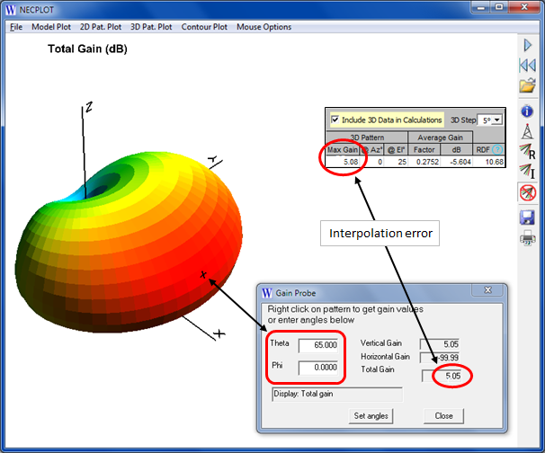
You can then either right-click anywhere on the pattern or set explicit Theta/Phi angles. The gain shown in the dialog window is interpolated from the surrounding four points so the displayed value will not exactly match the actual 3D pattern gain (5.05 dBi vs 5.08 dBi in this example). Using a smaller 3D step size will reduce the discrepancy.
As with 4nec2, the "$Temp$.out" file sent to NECPlotG/NEC5GI is an abbreviated form of a NEC engine output file. There is no wire data in the abbreviated file hence it is not possible to show wires on the 3D plot. That means that the Model Plot > Plot and 3D Pat. Plot > Model plot inset choices are not available
Note that the NECPlotG program is on the
NEC-4.2 CD. If you have the earlierNEC-4.1 CD you can get a replacement by sending an email to LLNL with the details of your $300NEC-4 license. THE NEC5GI program requires a separate $110NEC-5 license from LLNL.Saving 2D Slices: There may be times when you wish to show a 2D trace from a 3D pattern file and then overlay a second 2D trace from a different pattern file for comparison. In that case you can save either an azimuth or elevation "slice" from whatever is the currently-opened 3D pattern file.
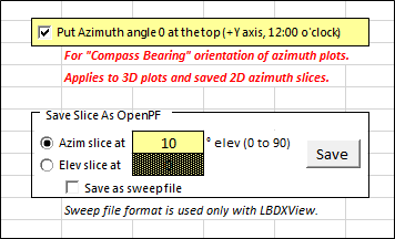
The OpenPF (*.pf) format is used with the EZNEC and 4nec2 viewers. The sweep file (*.txt) format is used with the LBDXView viewer. The NECPlotG and NEC5GI programs do not support overlay 2D traces.
For more information on antenna temperature and G/Ta see:
References
- Antenna Temperature Basics, DG7YBN
- TANT Manual and TANT Appendix, DG7YBN
- Effective Noise Temperature of 4-Yagi-Arrays for 432 MHz EME, DJ9BV, Dubus #4, 1987
- Performance Evaluation for EME Systems, DJ9BV and F6HYE, Dubus #3, 1992
- A G/T Study of Two Meter Yagi Antennas, VE7BQH, Dubus #1, 1996
- ITU Recommendation P.372-13 - Radio Noise, (available in multiple languages)
- G/T tables by VE7BQH, SM2CEW
- Ground Gain in Theory and Practice, ON4KHG, Dubus #3, 2011
- Caution Notes on Antenna Gain, W7GI
XLGTa is free but requires Excel 2000 or later. XLGTa does not work with other spreadsheet software such as OpenOffice Calc, LibreOffice Calc, Quattro Pro, Microsoft Works, or versions of Excel earlier than Excel 2000. None of these other spreadsheet programs fully support the macros used by XLGTa. Low-cost back-level versions of Excel (Office) can frequently be found on eBay (link).
DownloadXLGTa requires that Excel macros be enabled. Before opening the workbook for the first time you may scan it with your anti-virus program to assure yourself that it is safe. Then open it, enable editing, and enable macros. If you are not familiar with Excel workbooks containing macros you might want to look over Step 2 of this Quick Start Guide. That page was written for an application called AutoEZ but the same ideas are applicable to any workbook with macros.
To make the download file sizes smaller the initial workbook is loaded with a 3 degree step size file. When you load a 1 degree step size file you'll see
"Filling down more rows ..." in the Excel status bar area. If you then save the workbook with those extra rows added you can avoid the additional wait in the future. You should also save the workbook if you want to "remember" the most recent folders for reading *.pf3, *.csv, and *.13 files or to save your path settings for 3D viewers.For use with Excel 2007 and newer:
XLGTa_xlsm.zipFor use with Excel 2000, 2002/XP, 2003:
XLGTa_xls.zipAlso available are two "isotropic radiator" data files, both with 1 degree step sizes. One is in EZNEC pf3 format and the other is in MMANA csv format. When either is loaded you should see an Average Gain value of exactly 1, a T_loss value of exactly 0, and a T_total [Tant] value exactly equal to (Sum) T_pattern.
Isotropic.zipI am grateful to Jean-Pierre Waymel, F5FOD, and Hartmut Kluever, DG7YBN, for the detailed documentation and source code that they have provided. Without them showing the way the XLGTa tool would never have been created.
AcknowledgmentsI also appreciate the many helpful suggestions provided by Vladimir Kharchenko, UR5EAZ. His input made XLGTa much better than it would have been otherwise.
Thanks as well to the following for additional beta testing and feedback: KF6A, W8IO, G4CQM, N6LF, K7TJR, W8WWV, ON5AU, NC4FB, N7WS, OH2RA, OH6LI.
Models "DJ9BV_BVO_3wl.ez" (expand the AGTC_lite DEMO section), "G0KSC 432 LFA 22.ez" (using the dimensions shown), and "6m_8L_50ohm_yagi_kf6a.ez" (see model KF6A-50-8L in the 50 MHz table) were used in the illustrations above. All rights are reserved by DG7YBN, G0KSC, and KF6A respectively.
≈≈≈
Dan Maguire, AC6LA