Examples of using AutoEZ have been created from time to time to address questions raised on various forums and reflectors. This is a collection of such examples, in some cases slightly edited. Step by step instructions are omitted to maintain brevity.
Modeling for the N6LF "Elevated Radials" QEX article
A recent thread prompted me to re-read the N6LF QEX two-part article "A Closer Look at Vertical Antennas With Elevated Ground Systems", available here:
http://rudys.typepad.com/files/qex-mar-apr-2012.pdf
and here:
http://rudys.typepad.com/files/qex-may-jun-2012.pdfI created a general purpose model which may be used to duplicate many of the charts shown in the article as well as do other studies concerning elevated radials. Almost all aspects of the model are controlled by variables. I kept the N6LF usage for variables H, J, L, and N plus added a few others. The complete set is:
H: Vertical element length (may be 0 to model radials only)All dimensions are in feet. Variables T,U,V allow you to create a "T" or "Inverted L" radiator with either horizontal or sloping top wire(s).
J: Base height (may be 0 for use with Perfect or MININEC ground)
L: Radial lengths
N: Number of radials (may be set to 0, 1, 2, 4, 8, 16, or 32)
T: Top wire A (above +X axis) length (set to 0 for no top wires)
U: Top wire B (above -X axis) length (see below)
V: Angle of top wire(s), down from horizontalAs mentioned, one use of this model is to recreate the N6LF charts under different conditions. For example, here is Fig 12 from Part 1 of the article. In this case Average Gain is being used as a proxy for antenna efficiency. The length of the radials is swept from 0.05 λ to 0.6 λ and the chart shows a large drop in Average Gain as the radial length approaches 0.45 λ, less so when more radials are used.
Here's a similar chart, tailored for 160m, produced by AutoEZ.
Another example relates to the section "An Explanation for the Dips in Ga" (Part 1 pg 40) in which N6LF discusses the large current peaks that develop on the radials as the length approaches 0.45 λ. These large currents increase the E and H-field intensities in the ground. He then states: "Since the power dissipation in the soil will vary with the square of the field intensity, it’s pretty clear why the efficiency takes such a large dip when the radials are too long." This is illustrated with his Figs 24-26 (not shown here).
An alternate way of showing what is happening, not possible with a print publication, is to animate the E-field pattern as the length of the radials is increased. Here is the case for N=4 with the radial lengths ranging from L=0.05 λ to L=0.6 λ, the same range as the previous chart. Temporary variable "A" is being used to set the radial length in wavelength units which is then converted to the actual "L" in feet. Values for both A and L may be seen to the right of the chart. E-field was calculated at 1 foot below ground. With most browsers, press Esc to stop the animation in order to take a closer look at any frame, press F5 to restart.
Another way to use this model is for comparison between alternate scenarios. For example, W8JI suggested starting with two opposite radials trimmed to be a resonant dipole, then adding additional radials of the same length, then adding the vertical element and adjusting its length for feedpoint resonance. Modeling this scenario at 1.85 MHz, H=0 (no vertical element, to start), J=10 (base height), and N=2 (number of radials), the AutoEZ Resonate button yields radial length L=127.2 ft (0.24 λ) for "dipole resonance". Then with N=8 the Resonate button yields H=132.0 ft (0.25 λ) for a feedpoint Z of 39+j0 ohms.
Although the SWR is already low, to minimize feedline loss you might put a matching network at the antenna base. The AutoEZ Create Impedance Matching Network button allows you to easily add this to your model. With a Lo-Pass L network (coil in series, capacitor in shunt), the computed values are coil=1.804 µH and cap=931 pF to get 50+j0 ohms at the antenna. This is with real-world (lossy) components, assuming a coil Q of 200 and a capacitor Q of 1000, both at 1 MHz and adjusted as necessary for other frequencies.
Call this Scenario 1. For Scenario 2 suppose you have room for radials that are only 100 ft long, you can only get the top of the vertical up to 80 ft, and you'll add two top wires to make a "T" for the remaining radiator length.
With N=8, H=70 (puts the top at 80 with J=10), and U set to "=T" (that is, U will change as T changes so that symmetry at the top is maintained), the Resonate button sets T=42.8 ft to give a feedpoint Z of 25+j0 ohms. Then repeating the creation of a matching network, this time the computed values are coil=2.154 µH and cap=1684 pF to get 50+j0 ohms at the antenna.
Here's what the two antennas look like. Remember, both were created from the same model file, the difference is just how the variables were set.
Finally, how do the two scenarios compare? Here are the azimuth patterns at 22° elevation.
It's easier to discern the small difference in gain as well as the slight asymmetry of Scenario 2 when the pattern is shown in rectangular rather than polar format.
And here's the SWR comparison with the matching network in place in both cases.
The AutoEZ model can be downloaded (right click and select Save As) here.
Trimming Elevated Radials
A question was asked, "What is the preferred method of tuning elevated radials for uniformity?"
Lacking a good answer to the question about the preferred method of insuring uniformity in elevated radials I decided to look at the problem from the other direction. That is, intentionally make the radials non-uniform and then see what the difference in current magnitude/phase would be at the innermost point of each radial.
I started with EZNEC sample model ELEVRAD2.ez. This model was developed by W7EL to demonstrate the correct way to model radials close to ground, so the first thing I did was raise the entire model by 120 inches. With a 1 amp source the current distribution as shown by EZNEC is:
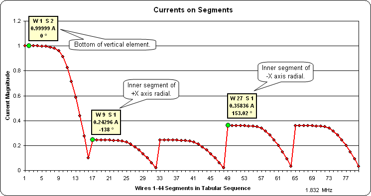
Looking at the same data charted a different way confirms the expected symmetry. The yellow "info boxes" show the Wire number (W), Segment number (S), current magnitude, and current phase for selected segments as marked with the green dots:
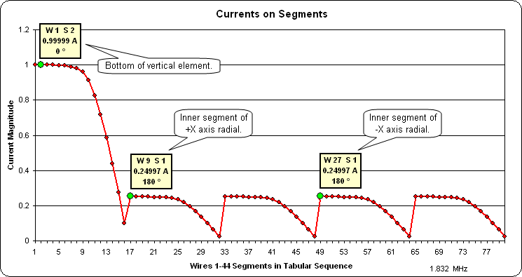
Note that in the above chart the "shapes" of the curves do not match what is shown in the EZNEC view. That's because in this particular model the segments do not have a uniform length. However, the magnitude/phase results are as expected; 1 amp at the source (Wire 1 Segment 2 [W1 S2]) and 0.25 amps at the inner end of each radial (such as Wire 9 Segment 1 [W9 S1]).
Next I modified the model to make the length of the two adjacent radials along the +X and +Y axes be 95% of the original length (1482" vs 1560" for the radials along the
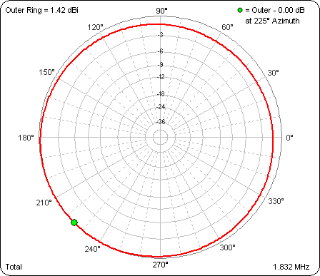
-X and-Y axes). As expected the radiation pattern is now a bit skewed. Here's the azimuth pattern at 24° elevation angle:
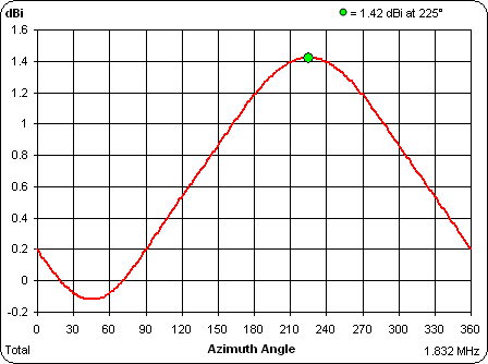
And here's the rectangular plot of the pattern instead of the polar plot:
The really interesting result is how much the current on the radials has changed given just a 5% difference in length. Wire 9 Segment 1 [W9 S1] is the inner end of one of the "shortened" radials, W 27 S 1 is the inner end of one of the original length radials:
Given the 47% change in the currents at the inner ends of the radials with just a 5% difference in lengths it seems reasonable that one could detect much smaller differences in "non-uniformity" of the radials using a simple current probe.
Elevated Radials - Near Fld Above/Below Ground
One poster mentioned a desire to compare an inverted L with elevated radials against a quarter-wave vertical with elevated radials. Another poster mentioned looking at the near field below the surface.
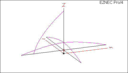
I put together a ".weq" format model for use with the AutoEZ program, with all dimensions controlled by variables. Here's a general view:
You can use this one model to study what happens when you change the height of the radials, the length of the radials, the length of the vertical section, and/or the length of the horizontal section. The horizontal section length may be set to zero in which case the model becomes a simple vertical. In the view above the radials are 130 ft (~87°), the vertical section is an arbitrary 65 ft, and the horizontal section has been set to ~71.9 ft using the Resonate button. Test frequency is 1.832 MHz. The AutoEZ model can be downloaded (right click and select Save As) here.
If you want to play with this model using the free AutoEZ Demo program you'll have to adjust the segmentation density down to roughly 20 segments per WL from the current 100 segs per WL. Use the AutoSeg button.
Finally, here's what the near field looks like at 1 ft above ground. This is looking straight down on the antenna. The color scale represents E-fld intensity.
And here's the E-fld at 1 ft below ground. This is not an apples-to-apples comparison; note the range of the scale is greatly reduced. (NEC4 engine required to produce this view.)