Examples of using AutoEZ have been created from time to time to address questions raised on various forums and reflectors. This is a collection of such examples, in some cases slightly edited. Step by step instructions are omitted to maintain brevity.
Doublet with Ladder Line Feed
The question is about how to do three separate things. First is to build an EZNEC model that matches the physical antenna system: an 88 ft doublet at 45 ft high fed via 110 ft of ladder line, then a 4:1 balun, then 8 ft of RG-8U coax to the rig.
That's relatively straightforward, at least after you've seen it done a few times. Here's the model.
When you open this model with EZNEC, look in the Sources window and note that the source is placed at virtual wire V1. Then in the Transmission Lines window there are two lines, the first (the 8 ft of coax) running from V1 to V2 and the second (the 110 ft of ladder line) running from V3 to the center of the antenna wire. The lengths are as specified by the original poster. The values for Zo, VF, and Loss can be obtained from a tool such as TLDetails or you can use values found in various publications. Note that the Zo of "450 ohm" ladder line is typically closer to 400 ohms.
The 4:1 balun is modeled as an ideal transformer. In the EZNEC Transformers window note that the connection is from V2 to V3 (between the two transmission line sections) and the impedance ratio is 1:4 between Port 1 and Port 2.
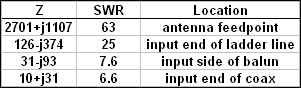
Including all the components of the antenna system in the model definitely makes a difference. For example, at a frequency of 21.225 MHz (center of 15m) here's how the impedance and SWR values change as you "work backwards" from the antenna to the station.
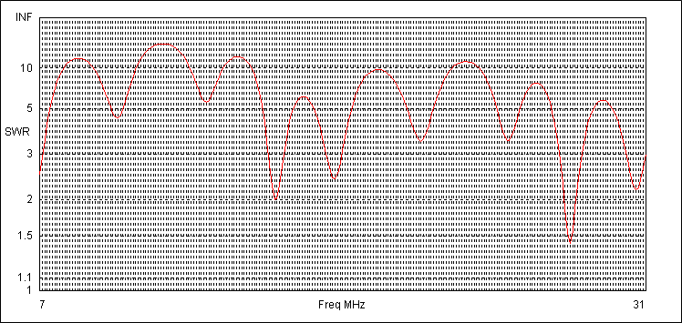
Because the source is at V1, when you run an SWR sweep the results will be as seen at the input (shack) end of the 8 ft of coax. Here's a sweep from 7 to 31 MHz. Note that the trace line is normally black. I changed it to red for this discussion.
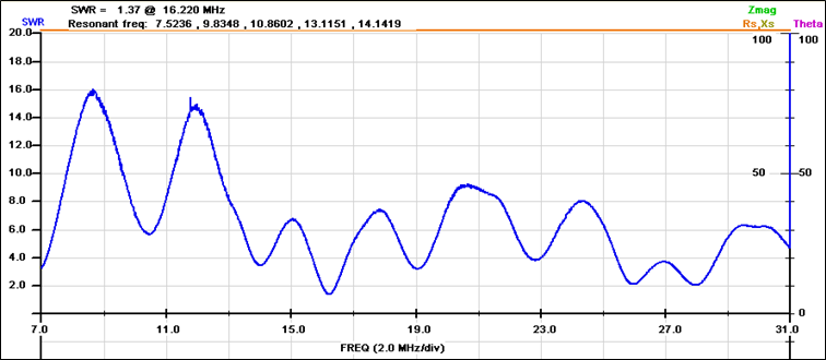
So far so good. The second question is to determine if the model matches the measured results using an AIM4170 device at the input end of the coax. Here's the AIM scan. This time I changed the SWR trace color from the normal red to blue.
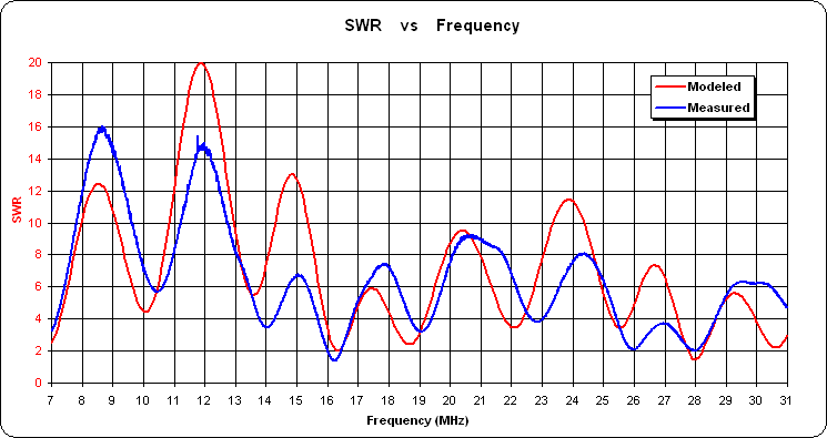
To make it easier to compare the two traces you can use the Zplots tool. Zplots can read both the measured data from the AIM device and the modeled data from EZNEC and show both traces on the same chart.
Note that when a linear scale is used for SWR the picture can be a little misleading. That is, the difference between SWR values of 2 and 3 is much more important than the difference between values of 12 and 13, but on a linear chart both show as the same vertical separation. A way to avoid that is to show the reflection coefficient (rho) instead. That's actually the way EZNEC shows SWR, namely a rho chart but with equivalent SWR gridlines. Here's the Zplots comparison showing rho instead of linear SWR.
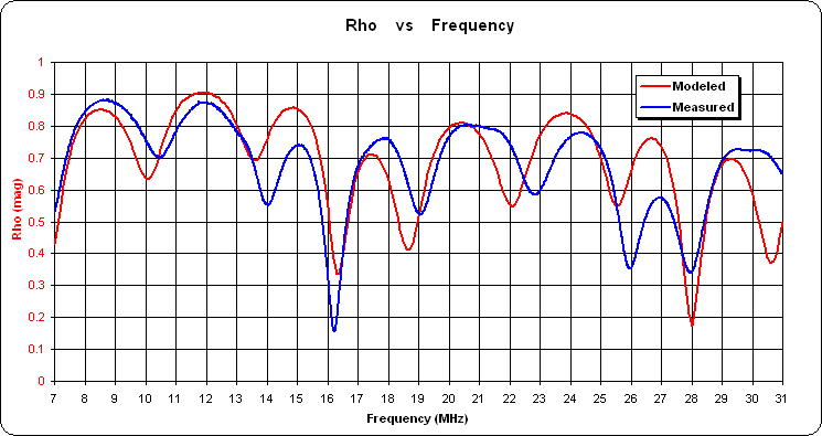
Looking at that chart it's clear that the modeled and measured results are at least in the same ballpark. If the antenna wire length and height are correct, the biggest unknown in the model is the ladder line. You could vary the modeled ladder line length, Zo, and/or VF, run a new SWR sweep, then load that new sweep data into Zplots to compare to the AIM measurements, tweaking things to try to get a better correlation. It would probably be easier to place a known load at the far end of the line, such as a 100 ohm resistor, model that with EZNEC, measure it with the AIM, and then adjust the ladder line characteristics until the two traces matched. But that's a discussion for another time.
Assuming that the model is at least a close approximation of reality, the third question is whether the total antenna system (doublet plus feed) can be modified to get a better match on 15m without having too much of a negative impact on the other bands. That kind of "what if" testing can certainly be done manually with EZNEC but an alternative is to use AutoEZ. AutoEZ acts as a driver for EZNEC and lets you modify the model using variables. For example, you could use variable "L" for the length of the antenna wire and variable "M" for the length of the ladder line. Then you could run a "variable sweep" instead of a frequency sweep.
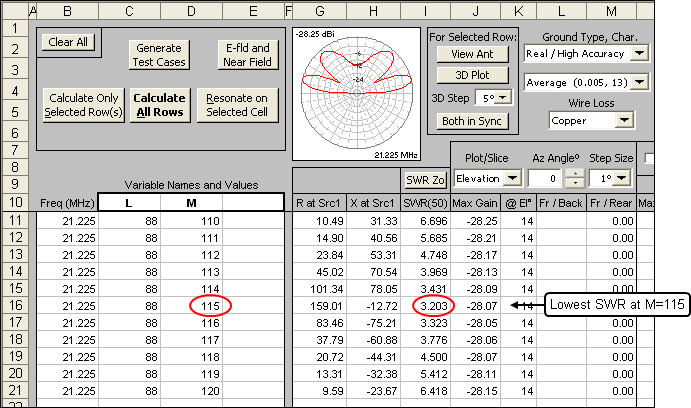
Here's an example of changing the length of the ladder line ("M") from 110 ft to 120 ft in 1 ft steps while keeping the antenna length ("L") constant, all at the mid-point of the 15m band.
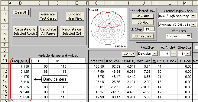
And this shows how you could keep both lengths constant while computing the results at the center of each band from 40m to 10m.
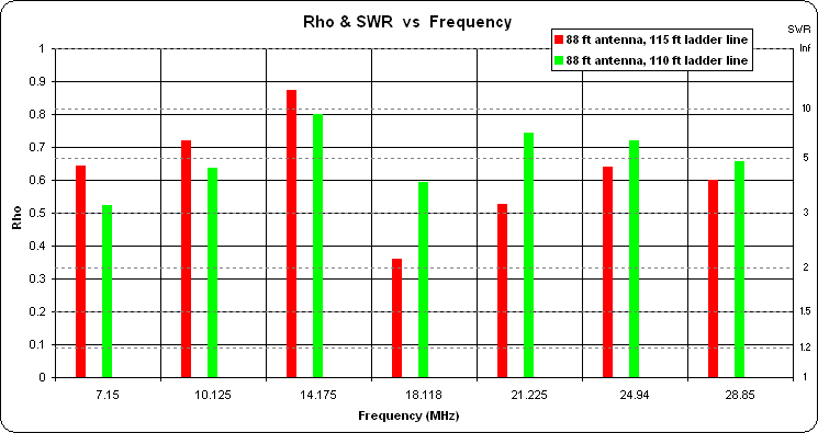
Besides numerical results AutoEZ also has several chart options that make "what if" comparisons easy. In this chart the green bars are with the original specs and the red bars are with the ladder line 5 ft longer. The chart shows both rho (left scale, solid gridlines) and equivalent SWR (right scale, dashed gridlines).
If you'd like to experiment with the free demo version of AutoEZ here's a model file you can use. (Note that you can't just click on the link to open the model. Save it to your computer then open it from within AutoEZ, as explained in Step 3 of the Quick Start guide.)
The model has been modified to have fewer segments so that it can be used with the demo. As a result you'll see EZNEC "Segmentation Check" warnings at the higher frequencies, which you can just ignore, and the calculated results won't be as accurate, which doesn't matter if you are just trying to get a feel for what AutoEZ can do. The model has variables for antenna length and height, ladder line length, coax length, and balun impedance ratio (1:1, 1:2, 1:4, 1:9, etc).
20m/15m Dipole
W5DXP posted an idea for a 20/15 dipole made from ~80 ft of wire fed with ~75 ft of ladder line. WA7DU said he'd like to try it but wouldn't know what do to with such a long run of ladder line.
Another option is to change the length of the dipole (doublet) which will result in both a different pattern and a different length of feedline. Here's a worked-out example using AutoEZ.
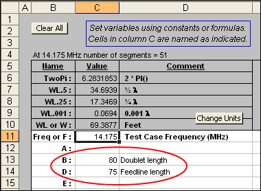
Starting with W5DXP's original specs of 80 ft for the antenna wire and 75 ft for the ladder line I defined two variables. Variable names "B" and "D" were used for this example but any names will do.
Then I created a single wire of length "B" at an arbitrary height of 40 ft.
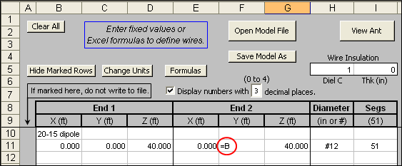
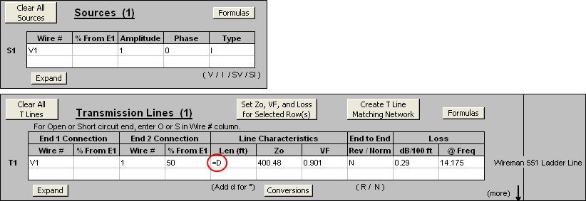
Next I created a transmission line of length "D" plus put the source on virtual wire "V1". So the connection sequence is V1 to transmission line to center of antenna wire (Wire 1 / 50%).
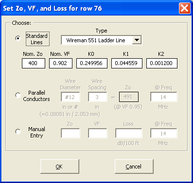
To set the Zo, VF, and loss characteristics of the transmission line I picked Wireman 551 from this dialog. You can choose from approximately 100 different standard line types or you can define you own wire diameter and spacing for parallel conductors.
Rather than try to manually pick various combination of "B" and "D", the equivalent of "trim and test" for real antennas, I let the AutoEZ optimizer calculate the exact antenna length and the exact feedline length that gives a combined minimum SWR at 14.175 and 21.225 MHz. This screen grab show the Optimize sheet tab after the run completed, which took 15 seconds. Note that the only optimization target was SWR, no attention was paid to Gain.
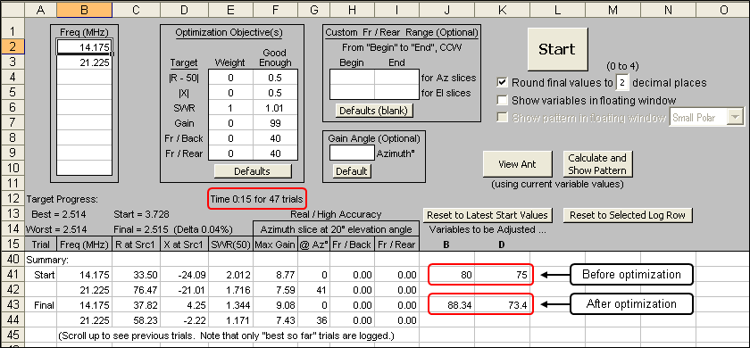
I then repeated the optimization but this time started with an initial value of 35 ft for variable "D", the feedline length. Starting at that point the optimizer "homed in" on a shorter antenna length (~61 instead of ~88 ft) as well as a shorter feedline length (~47 instead of ~73 ft). (Not shown.)
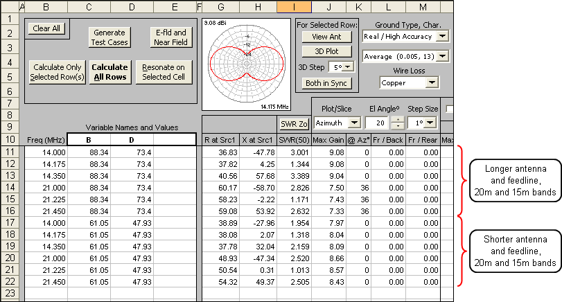
With those two sets of antenna and feedline lengths I set up a series of test cases. Each of the two "B" and "D" combinations was run against 3 frequencies in the 20m band and 3 frequencies in the 15m band.
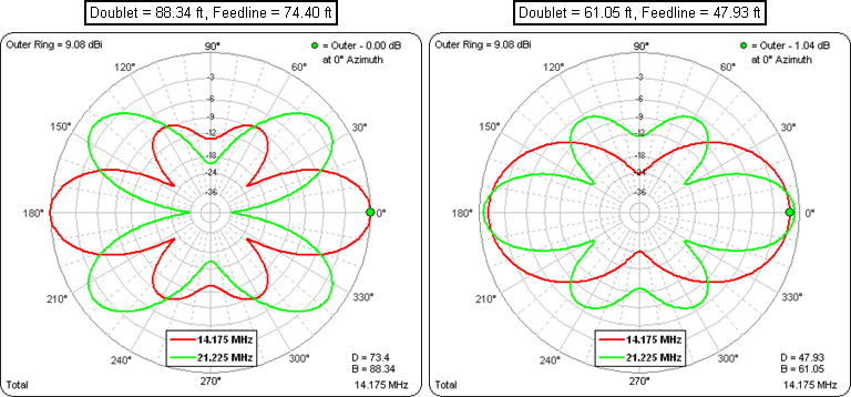
Here's what the radiation patterns look like. These are azimuth slices at an arbitrary take-off angle of 20 degrees. Red is for the middle of 20m and green is for the middle of 15m.
And here's a comparison of the SWR values for all six frequencies. This time red is for the longer antenna and feedline and blue is for the shorter combination. On 20m the shorter doublet with shorter feedline produces a wider bandwidth. At 15m the results are fairly similar.
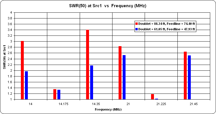
So, if you can live with the different pattern you can definitely eliminate some of the excess feedline.
Horizontal Loop for 160m through 10m
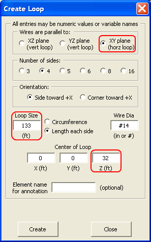
W6OGC asked if anybody was willing to model a horizontal loop for 9 bands, 133 ft on each side, 32 ft high, fed in a corner. Here is my reply.
I'll take that bait.
First I used this AutoEZ dialog to quickly create all four wires of the loop. Note that each side is 133 ft and the center is 32 ft above ground. Then just one click on the “Create” button does all the work.
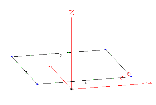
Here's the EZNEC view of the model. Don't be fooled by the viewing perspective, the loop really is square. The two red circles represent a "split" source which effectively puts the source at a corner, as requested.
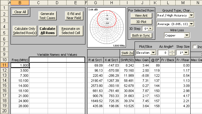
Then I set up and ran a series of AutoEZ test cases. This is a portion of the AutoEZ 'Calculate' sheet tab. Elevation plots are being requested. Note that the max gain, 7.87 dBi, happens at 18.1 MHz, at least for the 0 degrees azimuth angle at which the elevation plots were calculated.
After the calculations are done (only takes a few seconds) you can tab to the Patterns sheet and "watch the movie" of how the elevation pattern changes at each frequency. You can also create an animated gif of the patterns by using a combination of AutoEZ features and an external "Animated GIF Maker" program. Here's the animation. Note that the outer ring has been frozen at 7.87 dBi which allows for easy comparison of relative pattern strength as well as shape. Frequency is shown in the lower-right corner.
This animation loops continuously. When using AutoEZ directly you can stop and examine each frame as you wish. You can also take a "snapshot" of one frame and overlay it on another.
Then I redid the calculations, this time requesting azimuth plots at an arbitrary 20 degrees TOA. For this particular TOA the max gain was 13.33 dBi at 21 MHz. The outer ring is again frozen at that value to allow relative strength comparisons. Here's the movie for that.
40m Dipole with 15m "Capacity Hats"
W5DXP presented a version of a 40m dipole with added capacity hats to allow a better match on 15m. The idea is to use the same wire as both a 1/2 wave antenna on 40m and a 3/2 wave antenna on 15m, then add capacity hats 1/3 of the way along each side to improve the match on 15m without negatively affecting the match on 40m.
This is a classic configuration and the "rule of thumb" is to place the hats about 1/3 of the way out from the center insulator. In the configuration presented by W5DXP the "hats" were just single wires hanging down from the main span. In other versions the hats are made by twisting a closed loop of wire into a double loop and attaching the crossover point of that double loop to the main span. In that case the hats are sometimes referred to as "butterfly loops" since they resemble the wings of a butterfly with the attachment point being the butterfly's body.
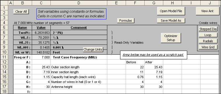
I couldn't resist running this model through the AutoEZ optimizer. Here's a screen grab after the optimizer finished. Variable "B" controls the outer section lengths (starts at 22 ft), variable "D" controls the inner section lengths (starts at 11 ft, hat attached here, total length each side 33 ft), and variable "E" controls the length of the 15m single wire "hats" (starts at 2 ft). The whole thing was modeled at 30 ft above Real-Average ground.
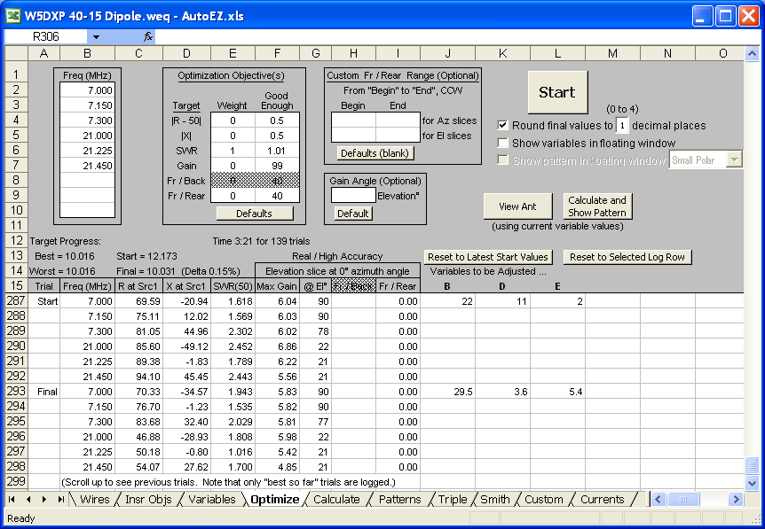
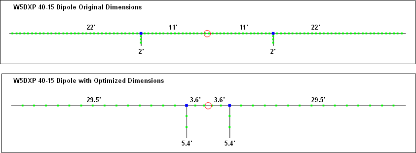
Turns out if the dimensions are adjusted as shown on the "Final" line (B=29.5, D=3.6, E=5.4), that is, move the hats closer to the center and make them a bit longer, you can get about the same match on 40 and a much better match on 15. The trade-off is slightly less gain, about 0.2 dB less on 40 and about 0.8 dB less on 15.
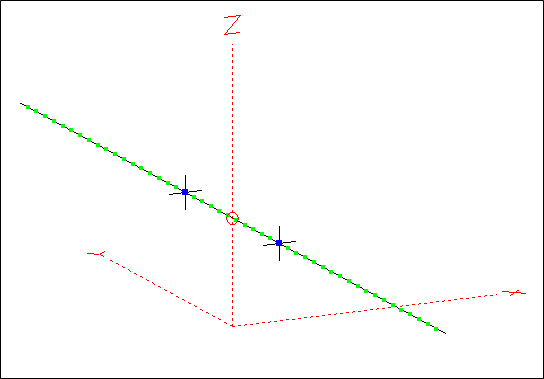
Here's a visual of the two models, which makes it obvious that the 15m part now resembles two inverted L's more than a dipole with hats:
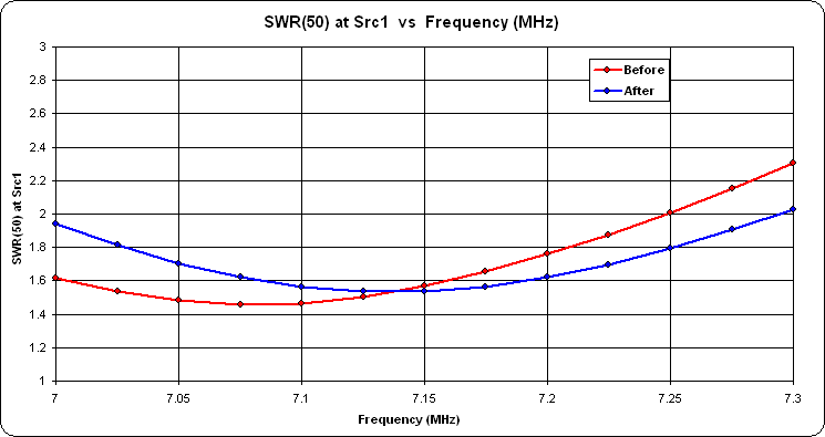
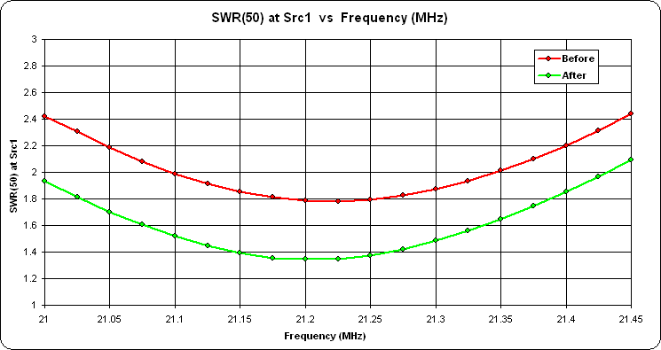
This chart compares the SWR curves on 40, before and after optimization:
And here's a similar comparison for 15:
In a later posting the geometry was changed slightly. Originally the capacity hats were modeled as just a single wire (each side) which led to some speculation that they were really acting more like separate "fans" of a fan dipole with a wide (long) common wire between the two sets of fans. So I decided to modify the model to make each hat four separate and opposing wires (like the letter "X"), more like a "real" capacity hat
Here is a screen grab of the "Variables" sheet from AutoEZ. Although it would be possible to do all of the necessary adjustments manually with EZNEC, it's much easier to just change a few variable values (or let the optimizer change the values) to reconfigure the model geometry.
The lengths of the eight hat wires (four on each side) were then adjusted to get the best match on 15m, leaving the position of each hat at 1/3 out from the center as "the books" suggest. That's the "Before" model. Then I used the AutoEZ optimizer to adjust the position of the hats, the size of the hats, and the overall length of the main wire, to get the best match on both 15m and 40m. That's the "After" model.
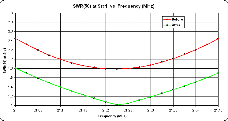
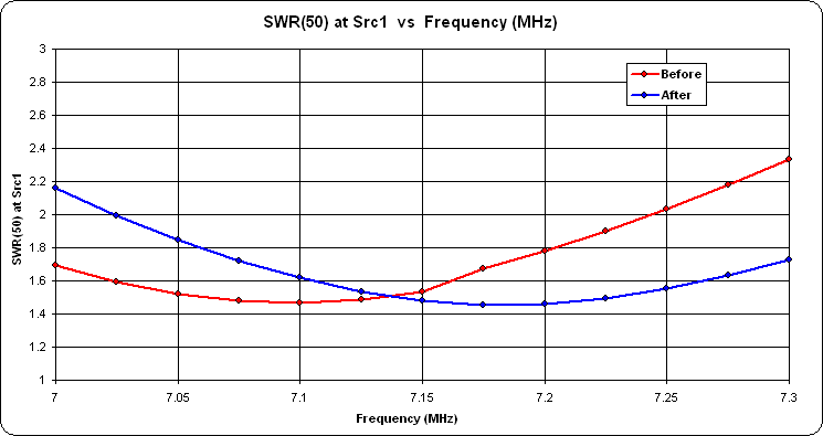
Here are the before and after SWR curves for 40m:
And here are the before and after SWR curves for 15m:
When using "real" capacity hats ("X" shape) the match on 15m isn't quite as good, SWR 1.35 vs SWR 1.02 with a "single wire" hat. However, unlike with that previous model, there is no change in the gain on 40m and only an insignificant drop of 0.05 dBi on 15m.
Here's the model file used in the above study. (Note that you can't just click on the link to open the model. Save it to your computer then open it from within AutoEZ, as explained in Step 3 of the Quick Start guide.)
Impedance and Length, 1/2 Wave vs 3/2 Wave
In a follow-up to the previous example of using the same wire as a 1/2 wave dipole on 40m and a 3/2 wave dipole on 15m, G3TXQ said "A 3/2 wave centre-fed has an impedance oscillating around 110 Ohms depending on height."
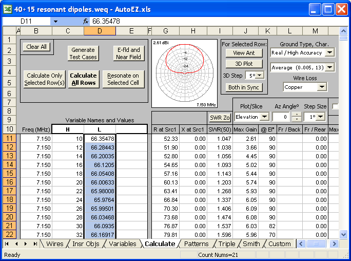
Using AutoEZ I modeled a 1/2 wave dipole for 7.15 MHz at various heights from 10 to 100 ft. For each step up in height I let the Resonate on Selected Cell button determine the exact length required for resonance (that is, X=0). In this screen grab variable "H" (column C) is the height and variable "L" (column D) is the length after being resonated.
Then I repeated the process at 21.225 MHz, this time for a 3/2 wave dipole. Here's a comparison of the feedpoint R value vs height above ground, produced using the AutoEZ 'Custom' chart sheet tab. As usual, G3TXQ's comment was spot on.
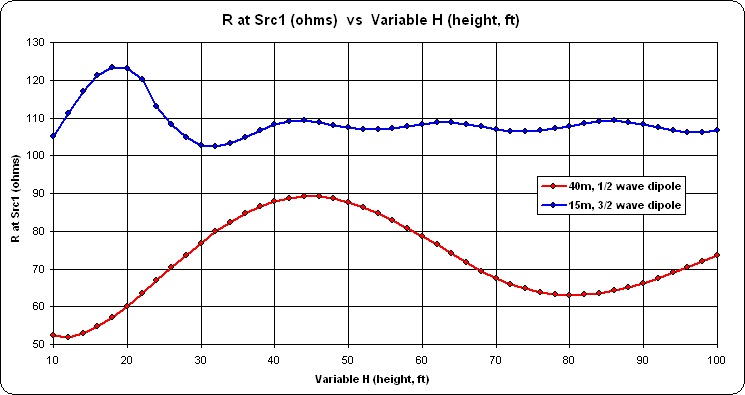
Normally you see charts like this with the horizontal axis being height in wavelengths, not feet. I chose feet to allow both curves to be shown on the same chart.
Another interesting chart is to plot resonant length vs height.
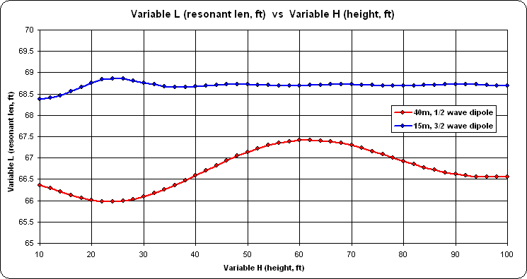
For the 40m points plotted, the average resonant length is ~66.7 ft. This is just slightly higher than the good ol' ARRL "cutting formula" of 468/F(MHz) for a half-wave dipole which would be ~65.4 ft at 7.15 MHz.
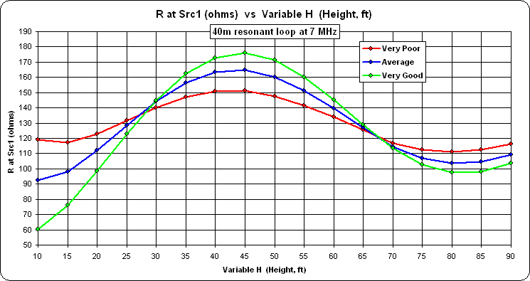
Horizontal Loop, Source R vs Height
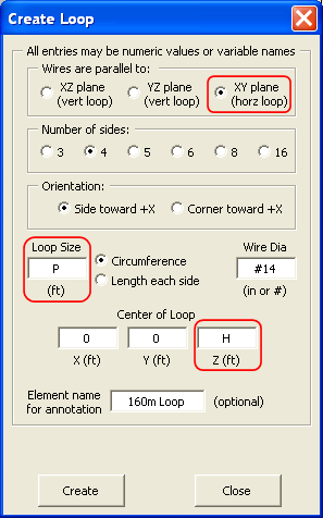
Here is an example similar to the previous one but for a 160m loop. With AutoEZ, I first used this dialog to create a 4-sided horizontal loop having a perimeter of "P" ft at a height of "H" ft above ground.
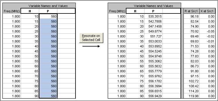
I then created a series of test cases with "H" ranging from 10 to 90 ft (~0.02 to 0.16 λ at 1.8 MHz) in 5 ft steps and with "P" having an initial value of 560 ft (~1005/Freq). Then the Resonate button was used to automatically adjust the loop perimeter "P" for resonance at each height.
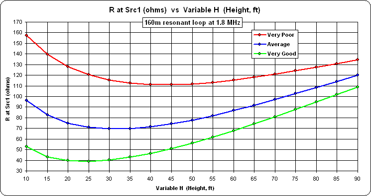
Repeating that process for three different ground types gives this result for the source resistance.
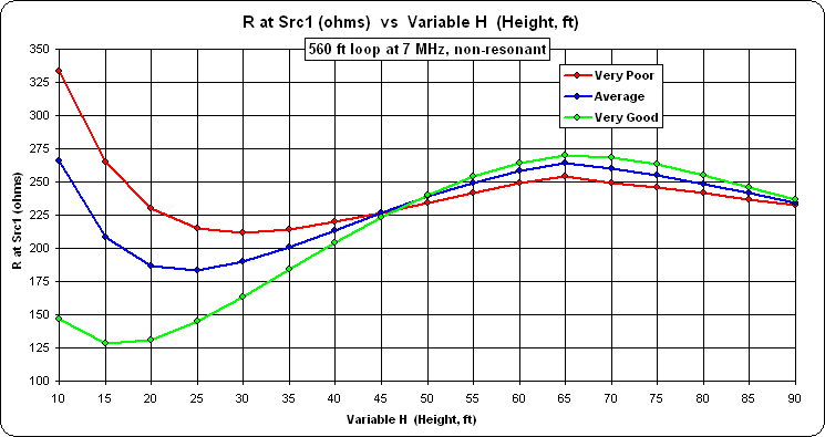
With the perimeter frozen at 560 ft, on 40m the loop will not be resonant. The source reactance will be a few hundred ohms negative. The source resistance will look like this.
On the other hand, if you calculate the source resistance for a 40m resonant loop, where the loop perimeter is ~145 ft and where 90 ft above ground is ~0.65 λ instead of ~0.16 λ, you'll get this.
If you'd like to duplicate these results, or run calculations for a different band, the following model file is suitable for use with the free demo version of AutoEZ.
Download that file, use the AutoEZ Open Model File button to open it, tab to the Calculate sheet, select all the "P" values (cells D11-D27), and click the Resonate button. Or change all the frequencies to your new choice and set all the initial "P" values to ~1005/Freq (initial value not critical), then click Resonate. Or just set all the frequencies and "P" values as desired and click Calculate All Rows instead of Resonate.
When the calculations finish tab to the Custom chart sheet. Select "R at Src" for the chart Y axis and "Variable 1" (which is "H", height) for the chart X axis.