Examples of using AutoEZ have been created from time to time to address questions raised on various forums and reflectors. This is a collection of such examples, in some cases slightly edited. Step by step instructions are omitted to maintain brevity.
20m Delta Loop on 5 Bands?
A question was asked if it would be possible to use a delta loop cut for 20m on all five upper bands (20/17/15/12/10) if the traditional quarter-wave section of 75 ohm coax were to be replaced with a 1:4 balun.
This whole scenario was modeled in just a couple of minutes with AutoEZ. First I used this dialog to quickly create all three wires of a delta loop, with arbitrary variable "D" for the circumference and with the center at 50 ft above ground. (Note that "C" is not available for use as a variable name.)
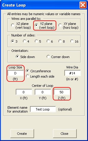
Variable "D" was given an initial value of 70 ft, roughly 1 λ on 20m. Then I used the Resonate on Selected Cell button to adjust variable "D" such that the loop would be resonant at 14.175 MHz.

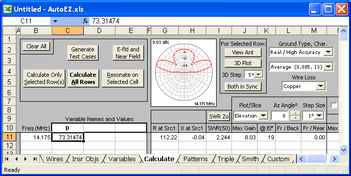
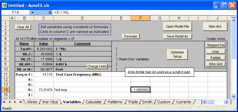
With Real-Average ground and copper wire loss that gave a loop circumference of ~73.3 ft which is about 1.057 λ. The 1.057 value was calculated just out of curiosity using the "scratch pad" area on the Variables sheet. In the screen grab below note that the formula in cell F14 is
"=D / WL" and "WL" is equal to one wavelength at 14.175 MHz. The value for "D" was set as a result of using the Resonate on Selected Cell button and the value for "WL" will automatically change as the frequency changes.
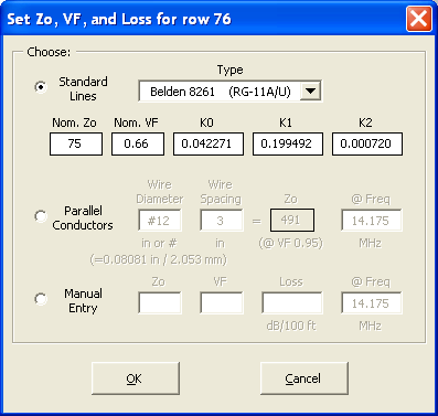
Then I added a quarter-wave section (Q-section) of 75 ohm line (Belden 8261, RG-11) to the model and moved the source from the center of the bottom wire to virtual wire 1 (V1).
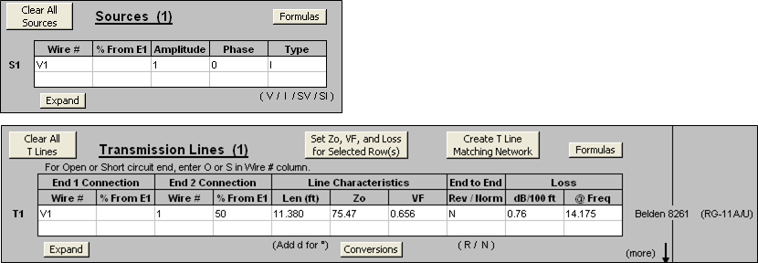
The exact values for Zo, VF, and loss (dB/100ft) for that type of line were set using this dialog, choosing from about 100 different built-in line types.
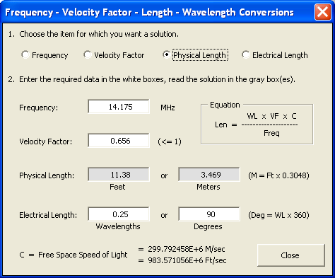
The length of the Q-section (11.380 ft) was determined using this dialog.
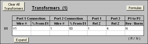
After running calculations at mid-band frequencies for 20/17/15/12/10 I deleted the Q-section and replaced it with a 1:4 balun, modeled as a transformer.
Now for the results. Here's the SWR at the mid-point of the 5 bands.
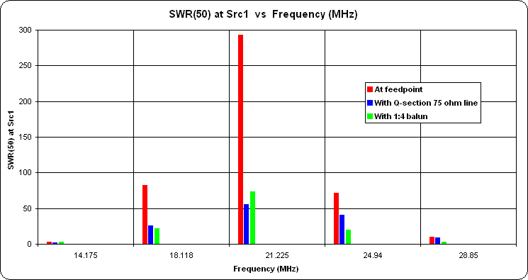
Obviously that's not a good way to look at things because of the huge SWR differences. A better way is to look at the reflection coefficient (rho) rather than SWR. Here's that chart, with various equivalent SWR reference lines added. For example, rho 0.091 is SWR 1.2:1 and rho 0.2 is SWR 1.5:1.
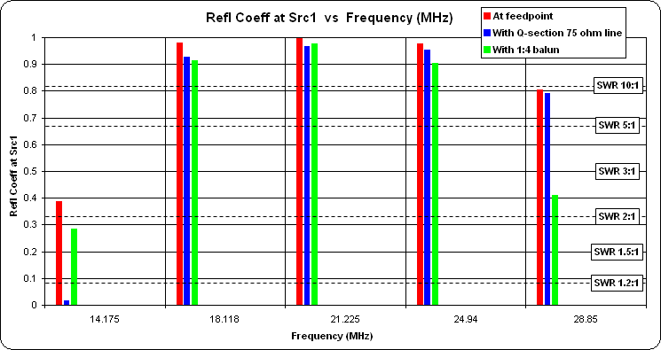
The only advantage of a 1:4 balun seems to be a better match on 10 meters, the trade-off being a much worse match on 20. As for all the other bands ... well, things don't look so good.
Multi-Band Vertical With Autotuner
In a discussion about multi-band vertical possibilities W5DXP showed this suggestion.
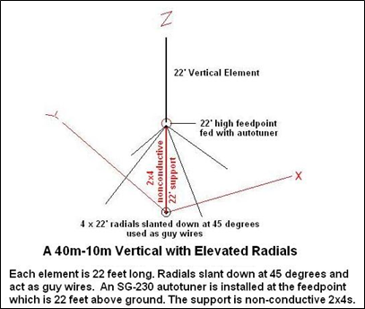
The W5DXP page mentions that his antenna is fed via an SGC-230 autotuner. AutoEZ can simulate autotuners so I thought I'd give this a shot.
First item of business was to create a model of just the antenna itself with all aspects controlled via variables: base height, length of vertical element, length of radials, diameter of vertical and radials, number of segments in vertical and radials. You could use this model to play "what if" with various dimensional changes even if you are not interested in simulating an autotuner. (See end of this example to download model files.)
With the base at 22 ft and the vertical and radials at 22 ft in length, here's an animation of how the pattern changes for each band. The frequency is shown in the lower right corner. (With most browsers, press Esc to stop the animation, F5 to restart.)
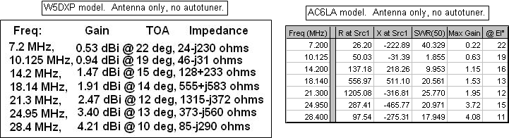
And here are the values for the feedpoint impedance, max gain, and TOA. The values do not match the W5DXP numbers because I used 22 ft for all elements, as shown in the illustration, whereas Cecil's table values are based on a model with a 22.25 ft vertical length and 21.92 ft radials.
Average ground was used for the above calculations. The difference between Very Poor and Very Good ground amounts to about a 3 dB change in max gain. For example, here's what the pattern at 28.4 MHz looks like with different grounds. Contrary to what might be expected, in this particular case the max gain is actually better with Very Poor ground.
Next it was time to model the autotuner. An autotuner differs from a regular tuner in that a) the L and C values change in discrete steps (controlled via relays) as opposed to being continuously adjustable and b) the L and C values change automatically as the frequency, and hence the impedance to be matched, changes. For the model, AutoEZ can do all the math to calculate L and C for a match, set L and C to the closest "step" value, and change the L and C values for each frequency, just like a real autotuner.
Reading the SGC-230 user manual it appears that the L step size is 0.25 µH and the C step size is 25 pF. Telling AutoEZ to build such a tuner and then running the test cases shows a pretty good match except at 28.4 MHz. Besides the SWR note the difference in the max gain values. That difference represents the loss in the tuner, assuming an inductor Q of 200 and a capacitor Q of 1000, both at 1 MHz and frequency adjusted.
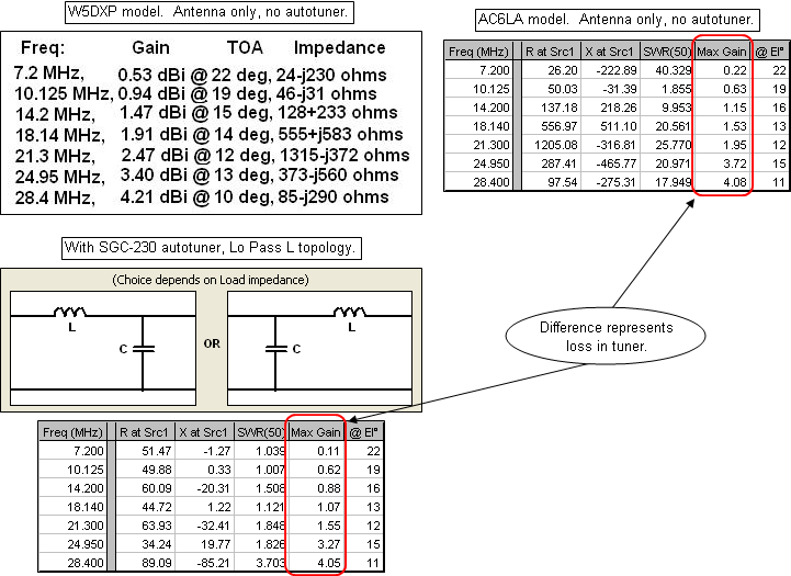
One thing that wasn't clear to me after reading the SGC manual was whether the tuner topology was a Lo Pass L (like most autotuners) or a Lo Pass Pi. If the SGC is a Lo Pass Pi topology then the match gets better at 28.4 but worse at some of the other frequencies. Note that to simulate a Lo Pass Pi network with EZNEC you actually use back-to-back L networks, automatically built by AutoEZ. (It could be that the SGC-230 is really some kind of composite topology that AutoEZ can't automatically simulate, requiring some manual modifications to the network.)
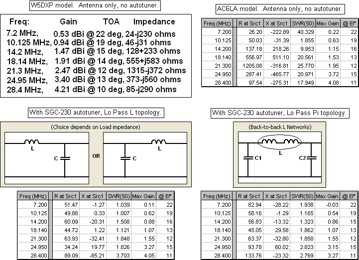
Here's a different way of looking at things, showing the SWR. In the second chart the scale max has been set to 5 to allow better comparison of the two different networks types.
This is the ".weq" format model (antenna only) to be used with AutoEZ. (Note that you can't just click on the link to open the model. Save it to your computer then open it from within AutoEZ, as explained in Step 3 of the Quick Start guide.)
And here's the same model with an autotuner (Lo Pass L topology) included.
The part of the AutoEZ User Guide that discusses modeling an autotuner may be found in the "Simulate an Auto-Tuner" section of the "Transmission Lines - Tuners - Stacks - Stubs" page.
NVIS Performance vs Quality of Ground
A question was asked about performance of a low 80m dipole intended for NVIS operation.
Here's the polar pattern with the dipole at a height of 10m (1/8 λ) for Very Poor and Very Good ground, per EZNEC definition of such. Average ground would be in between. Note the outer ring is 7.20 dBi. The green dot marker shows that there is roughly a 3 dB difference in overhead gain.
Just to round out the topic, here's how the pattern changes as the antenna is raised from 10m (1/8 λ) to 80m (1 λ). Average ground was used for this scenario. The height above ground is shown in the lower right corner as H=xx in meters. The outer ring is frozen at 8.18 dBi which is the max gain at 50m, the highest gain (at any take off angle) of the 8 patterns. That lets you compare the absolute gains as well as the pattern shapes. Also, the green dot marker is automatically placed at the max gain point for each separate pattern. If you look in the upper right corner you can see how the take off angle gets lower as the dipole is raised. (With most browsers, press Esc to stop the animation, F5 to restart.)
And here's the same scenario but in rectangular format.
Response of Fixed-Component L Network
A conjecture was made, "It seems like the input of a [fixed-component] matching network would have the same property of variation in input impedance [compared to the network output impedance] across a range of frequencies."
This scenario is relatively straightforward to model. Here's an example using AutoEZ.
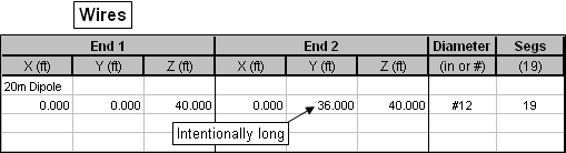
The first step is to create the wire for a simple 20m dipole. In keeping with an earlier comment that the intent is to lower the antenna and trim it once the snow melts, the length of the wire has been intentionally made a bit too long. Height is set at an arbitrary 40 ft in this example.
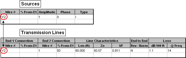
Next put a source on virtual wire "V2" (any virtual wire number would do, from 1 to 999) and define a transmission line running from V2 to the center of the antenna wire (Wire 1/50%). The length of the transmission line is set to 60 ft, again just an arbitrary choice.
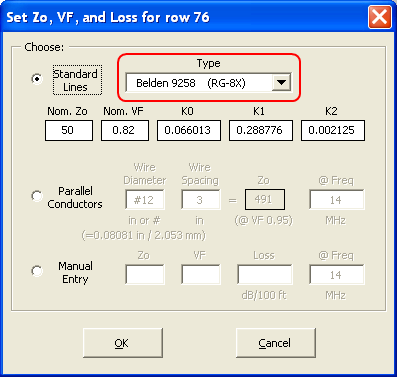
The remaining fields (to the right of Len) for the transmission line can be set with this dialog, which lets you choose from about 100 different built-in line types.
RG-8X was used just as an example. Note that the values for Zo and VF shown above are slightly higher and lower, respectively, than the “nominal”RG-8X values. AutoEZ will automatically recompute Zo and VF, as well as loss, to be accurate at any frequency.
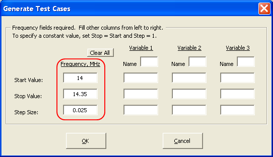
On the Calculate sheet use this dialog to generate a set of test cases, in this example just a simple frequency sweep.
Here are the calculated results. Note that the R/X values are as seen at the input end of the transmission line since that is where the source has been placed.
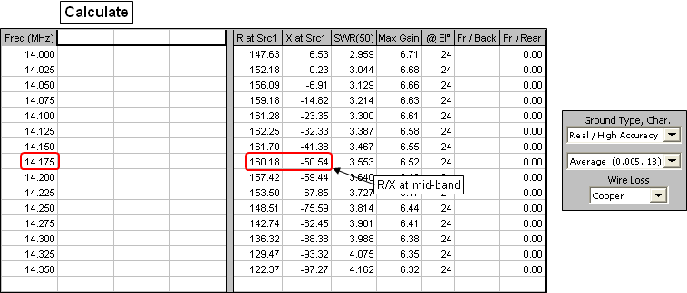
With the R/X values at the input end of the transmission line now available, the final step is to create an impedance matching network. In this example a simple "Lo Pass L" network with one coil and one capacitor is used. You can also create Hi Pass T, Lo Pass Pi, and Hi Pass L networks. In the lower part of the dialog window note that the network component values will be set to produce a match to the transmission line input impedance at 14.175 MHz, as calculated in the previous step. That is, the network values (coil µH and capacitor pF) will be set such that
160.18-j50.54 ohms is transformed to50+j0 ohms.
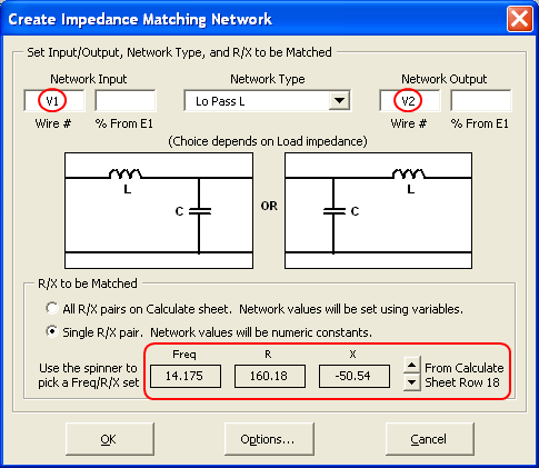
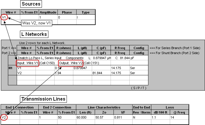
In the above dialog virtual wire "V1" was set as the network input and "V2" as the output. So the only thing left to do is move the source from its current position of V2 (the input end of the transmission line) to V1 (the input side of the network).
Recalculate to get new results with the network in place. Here's what the SWR looks like across the 20m band. I used the Snapshots button to capture the other traces at intermediate stages of building the model.
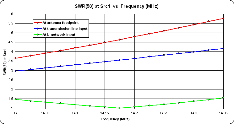
And here are the same results on a Smith chart. The light green circle shows 2:1 SWR.
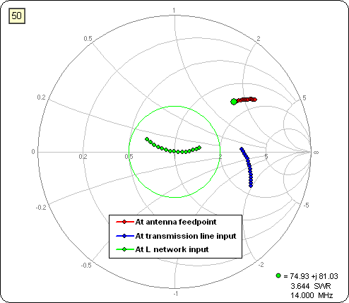
With the above two plots you can compare how the response varies at the network input side (green trace) as opposed to the network output side (blue trace).