A popular antenna system, especially on the lower HF bands, consists of multiple elements all driven directly via feedlines. One implementation of such a system uses lines of different lengths to provide the proper current magnitude and phase to each element. This section will explain how to use Zplots to "see" what is happening along the lines.
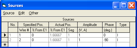
The example used is an EZNEC model of a simple two-element cardioid array at 7.15 MHZ and is discussed in more detail in Chapter 8 of recent editions of The ARRL Antenna Book. Each element is a quarter-wave ground-mounted vertical, spaced a quarter-wavelength apart, fed with equal amplitude but 90° out-of-phase currents. The elements are 33 feet tall and would be self-resonant (have zero reactance) if operated in isolation. Rather than model any buried radials directly (which would require use of a NEC-4 engine), Real/MININEC type ground is used and a lumped load is added to the base of each element. To simulate the approximate effect of 8 buried radials the load value is 18 ohms. This adds 18 ohms of loss resistance in series with the element's radiation resistance.
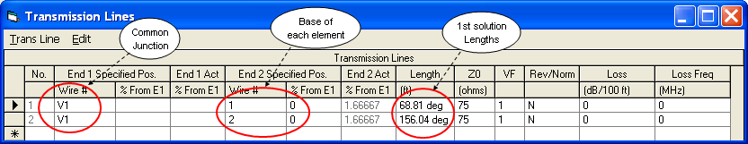
The relevant EZNEC panels are shown below.
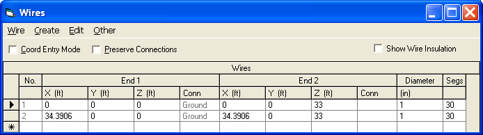
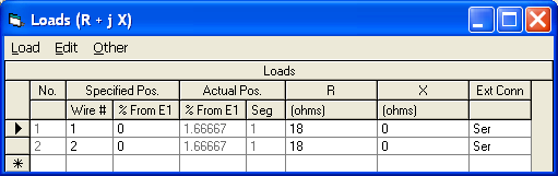
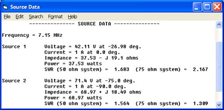
Note that if either element were operating independently the source impedance would be approximately 54+j0 ohms, a combination of 36 ohms radiation resistance and 18 ohms of ground loss. Because of the mutual coupling between the elements the two source impedances differ from this value, and because the elements are driven 90° out-of-phase the source impedances differ from each other.
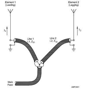
The initial model uses ideal current sources at the base of each element to provide the correct current magnitude and phase. But the ultimate goal is to feed the elements via lines of different lengths from a common junction while still providing equal magnitude and 90° out-of-phase currents. This is shown at left in an illustration from The ARRL Antenna Book (Fig 16 on pg 8-18 of the 21st edition). For reasons not covered here the phase delays introduced by the separate feedlines (Line 1 and Line 2 in the illustration) are not equal to the electrical lengths of the line. That is, you can't just make Line 2 90° longer than Line 1 and expect the current at the base of element 2 to be equal in magnitude but 90° behind in phase compared to that of element 1.
What you want is two separate lines that will provide the correct current magnitude and phase at their load ends while having equal voltage magnitudes and phases at their input ends so that they can be joined together at the common junction point. So how do you know how long to make each line?
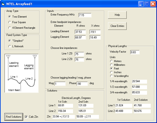
Roy Lewallen, W7EL, has written a utility program called Arrayfeed1 to do the necessary calculations. Use of this program is explained in great detail both in the help file and in Chapter 8 of the 21st and later editions of The ARRL Antenna Book. Without repeating the details here, basically you enter the feedpoint conditions for each element and the characteristic impedance (Zo) of each feedline. The program will calculate the electrical length in degrees for each line. If you've entered a Velocity Factor (VF) you'll also be shown the physical length that corresponds to each electrical length.
In general the Arrayfeed1 program will tell you everything you need to know. But what if you want to actually visualize what is happening along the length of each line? That's where Zplots can help.
|
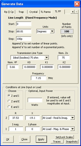
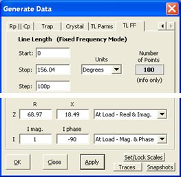
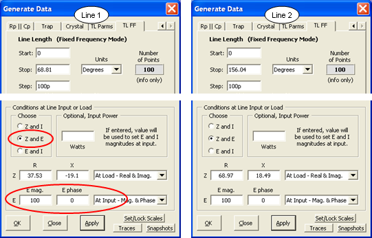
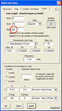
At left is the Zplots "TL FF" (Transmission Line at Fixed Frequency) Generate Data setup for Line 1. The entries in the top portion (namely a section of 75 ohm line that is 68.81 electrical degrees in length) correspond to the values from the Arrayfeed1 program. The entries in the bottom portion (impedance of Even though you set the current at the load what you want to see is the voltage magnitude and phase along the length of the line. Choosing "E-mag (V)" and "E-phase (deg)" for the left and right trace selections will produce the chart below. 
|
Although the line length is 68.81 degrees the scale for the X axis of the chart has been set to a span of 0 to 80 degrees. This was done merely to provide nice round numbers for the vertical gridlines.
At the load end of the line (towards the right) notice that the values for the voltage magnitude (red trace) and voltage phase (blue trace) match those shown by EZNEC for source 1 at the base of element 1. Following both traces to the left (towards the input end of the line) you can see how the magnitude and phase change.
Repeating the process for Line 2 as shown below (this time with the X axis spanning 0 to 160 degrees) yields a completely different looking set of traces for voltage magnitude and phase. But notice that the conditions at the input end of Line 2 are exactly the same as at the input end of Line 1. Hence the lines may be joined together at that point.
|
|
You can use the "Snapshots" button to display both sets of traces at the same time. That is, with the Line 2 traces being shown take a snapshot of both. The red trace will be overlaid with a green snapshot and the blue trace will be overlaid with a cyan (light blue) snapshot. Then re-plot for the Line 1 conditions.
This gives a "picture" of what is happening. At the input ends of the lines the voltage magnitudes and phases are equal so the lines can be joined together. At the load ends of the lines the voltage magnitudes and phases are completely different, yet they produce the desired current magnitudes and phases needed to give the correct antenna system radiation pattern.
As shown below, you can create a similar chart for the "2nd Solution" line lengths provided by Arrayfeed1.
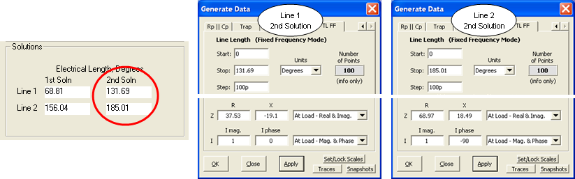
Notice that the conditions at the load ends of the lines are identical to the 1st solution. Hence the same currents would be produced in the antenna elements. However, this time the common value at the input ends of the lines is 73.10 V at 109.97 deg.
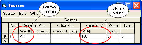
Now it's time to change the EZNEC model by deleting the two ideal current sources, adding two transmission lines, and adding a single source at the common input ends of the transmission lines. In actual operation the magnitude of the voltage and current at the common junction would depend on the power supplied by the transmitter. For modeling purposes any value will do. In the example below a voltage source of 100 V at 0 deg has been arbitrarily chosen.
This example also uses a "virtual segment" (V1) at the common junction. Virtual segments are a feature of EZNEC v.5. If you have an earlier version of EZNEC just use a very short wire that is positioned at some point between the two antenna elements.
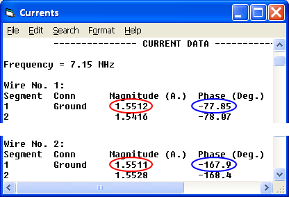
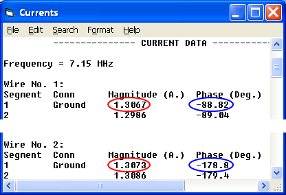
To verify correct operation take a look at the EZNEC "Currents" window. The current magnitudes (circled in red) at the base of each element are virtually equal. The phases (circled in blue) differ by the desired amount, with element 2 lagging by 90° compared to element 1.
And to "see" what's happening with the currents in the two transmission lines:
This time the voltage is set to the common arbitrary value at the input ends of the lines.
The chart at left was created by first plotting the conditions for Line 2, choosing "I-mag (A)" and "I-phase (deg)" for the left and right trace selections, setting the X axis to a span of 0 to 160, taking snapshots, then plotting the conditions for Line 1. (Line 2 was plotted first merely so that the legend entries would appear in Line 1 - Line 2 order.)
The current magnitudes (red and green traces, left scale) have the same value at the load ends of the lines, as desired. The current phases (dark blue and light blue traces, right scale) differ by the desired 90 degrees.
Throughout this entire example the line lengths have been expressed in units of electrical degrees. That makes the lengths valid at only a single frequency, in this case 7.15 MHz. If you want to see how this antenna system would perform over the entire 40 meter band you'll have to express the line lengths in physical units such as feet. The Arrayfeed1 program can do the conversion if you supply a velocity factor value.
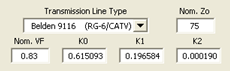
You might be tempted to use a "nominal" VF value such as 0.66 for solid polyethylene dielectric lines, 0.7 for Teflon dielectric, or 0.83 for foamed polyethylene. But keep in mind that both the velocity factor and the characteristic impedance Zo change slightly with frequency. For example, suppose you decide to build your phasing lines using "RG-6 CATV" coax purchased from a Lowe's Home Improvement store. Over a range of 1 to 100 MHz the actual Zo magnitude and VF look something like this:
As the frequency decreases, notice how the Zo magnitude (red trace, left scale) rises from its "nominal" value of 75 ohms while the velocity factor (blue trace, right scale) drops from its nominal value of 0.83.
For this particular example, using 75.613 instead of 75 for Zo in Arrayfeed1 changes the electrical lengths by a few tenths of a degree. Using 0.8234 instead of 0.83 for VF changes to the physical line lengths by a few inches.
|
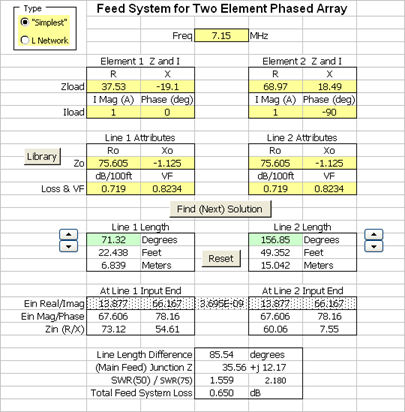
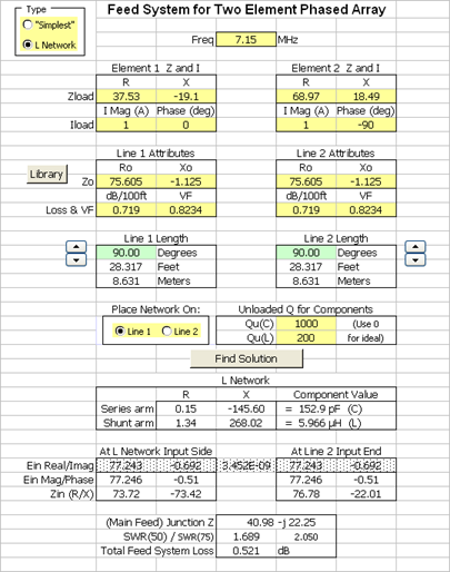
You can take this analysis of "real world" lines a step further if desired. Arrayfeed1 assumes ideal (no loss) lines and scalar values for Zo such as 75 ohms. I was curious to see what the effect would be of using lines that have both loss and a complex Zo so I created the Feed2EL Excel workbook. The partial screen grab at left shows the results and here's a summary of the findings:
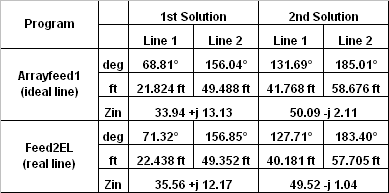
When using "real world" lines there is definitely a difference in the solutions. But what effect would these differences have on the current magnitude and phase at the base of each element? And how would this antenna system perform over the entire 40 meter band when using such lines? |
To answer those questions the first step is to modify the EZNEC transmission line specifications, as follows.
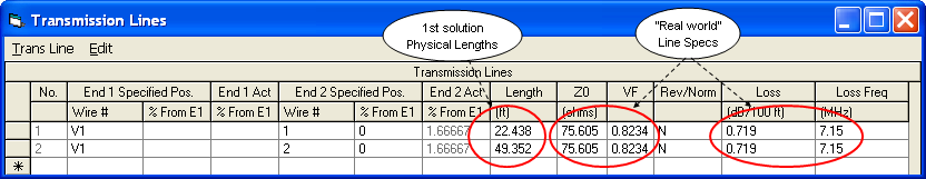
Note that when specifying lossy transmission lines with EZNEC you should use the Ro value in the EZNEC "Z0" column. EZNEC will calculate the correct Xo value under the covers.

This time the current magnitudes (circled in red) at the base of each element are slightly smaller because of the line loss, although they are still virtually equal as desired. And the phases (circled in blue) still differ by the desired amount, with element 2 lagging by 90° compared to element 1.
So far the discussion has been limited to a single frequency, 7.15 MHz. But what happens if the antenna, now fed via transmission lines having fixed physical lengths and with losses included, is operated over the entire 40 meter band? And since there are multiple combinations of feedline lengths that produce the same ratio of currents at the element bases, what criteria should be used to choose between the alternate solutions? Notice that the 2nd solution (for "real world" lines) produces an impedance at the line junction of
49.52-j1.04 ohms. That would provide an almost perfect match to a standard 50 ohm transmission line, so why not just use that one?This issue is discussed in both the Arrayfeed1 help file and in Chapter 8 of the 21st and later editions of The ARRL Antenna Book. Essentially the same wording is used in both and here's a direct quote from the help file:
Although it’s tempting to select the solution providing the best impedance match to the main feedline, this isn’t a good criterion to use. Usually, it’s best to choose the solution in which the difference in electrical lengths between the lines is closest to the phase delay of the currents between the elements. This will usually result in an array whose pattern and impedance are less sensitive to frequency and physical array variations. Impedance matching can be done at the main feedpoint as necessary.For the 1st solution the difference between the line lengths is about 85 degrees. For the 2nd solution it's about 55 degrees. So let's see how the two solutions perform across the entire 40 meter band.
Sure enough, the SWR for solution 1 (red trace) is fairly flat across the entire band. Solution 2 (green trace) is not quite as flat but (in this case) shows lower overall values. And although either one would be entirely acceptable in practice, just for illustration I added a simple impedance matching network between the solution 1 junction point and the main feedline. The SWR response for that combination is shown as the magenta trace.
I used a simple L network for the impedance matching but you could do the same thing with a series-section transmission line transformer, a stub match, or various other techniques. See Chapter 26 of The ARRL Antenna Book for more details.
The real difference between the solutions shows up in the pattern. Although the forward gain is almost the same in both cases (and won't be shown here), the F/B ratio is again flatter for Solution 1.
Note that the inclusion of an impedance matching L network at the junction has no effect on the pattern. There is no need to show a third (magenta) trace because it is exactly the same as the red trace.
If you'd like to experiment with an analysis similar to the above, the EZNEC model files (.ez) are available at Sample Feed2EL Models.zip. Note that most of the models make use of virtual segments, lossy transmission line, and/or L networks. Hence they must be used with version 5 of EZNEC.
It's interesting and enlightening to do theoretical studies like this but there's no point in going overboard with precision. Remember that everything is based on the impedance values at the feedpoints for each element. Even the best of models will probably be off by at least a few ohms. The only way to know for sure is to do actual measurements while the antenna is in operation. Chapter 8 of The ARRL Antenna Book describes methods to do just that.
Before ending this discussion of phasing lines there's one other item to mention. An alternate method to feed the two elements of the antenna described above is to use an L network to provide the necessary phase delay and then two quarter-wave "current forcing" transmission lines to feed the elements. (Note that this network is not the same as the L network mentioned previously. That one was for impedance matching and was inserted at the end of the main feedline. The one described here is for phase shifting, not impedance matching, and is inserted before one or the other of the "current forcing" lines.)
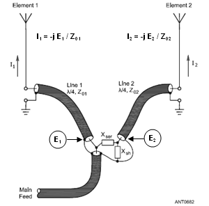
This alternate feed method is shown at left in an illustration from The ARRL Antenna Book (Fig 17 on pg 8-19 of the 21st edition, with additional annotation added). The L network, consisting of series reactance Xser and shunt reactance Xsh, provides a desired ratio between voltages E1 and E2. The action of the "current forcing" transmission lines then reproduces this same ratio in the currents at the base of the respective elements, assuming Z01 equals Z02.
Why is that? And what do the voltage and current magnitudes and phases "look like" on the transmission lines?
First the math. The general equation (Terman, Radio Engineers' Handbook and others) relating the voltage at the input end of a line to the voltage and current at the load end is:
Ein = Eload * cosh(gamma*len) + Iload * Zo * sinh(gamma*len)where:Ein = Voltage at inputThe complex propagation constant gamma is composed of a real part, alpha, and an imaginary part, beta. That is:
Eload = Voltage at load
Iload = Current at load
Zo = Characteristic impedance of the line
gamma = Propagation constant of the line
len = Line length
Note that all quantities except the line length are complex.gamma = alpha + j betawhere:alpha = attenuation constant, nepers per unit lengthThe complex hyperbolic functions cosh(gamma*len) and sinh(gamma*len) can be broken down into a sequence of scalar functions as follows:
beta = phase constant, radians per unit lengthcosh(gamma*len) = cos(beta*len) * cosh(alpha*len) + j (sin(beta*len) * sinh(alpha*len))For a lossless line the attenuation is 0 so alpha*len is 0. For a quarter wavelength beta*len is pi/2 radians or 90 degrees. So the cosh(gamma*len) and sinh(gamma*len) expansions become:
sinh(gamma*len) = cos(beta*len) * sinh(alpha*len) + j (sin(beta*len) * cosh(alpha*len))cosh(gamma*len) = cos(90°) * cosh(0) + j (sin(90°) * sinh(0)) = 0 * 1 + j (1 * 0) = 0 + j0Therefore:
sinh(gamma*len) = cos(90°) * sinh(0) + j (sin(90°) * cosh(0)) = 0 * 0 + j (1 * 1) = 0 + j1Ein = Eload * (0 + j0) + Iload * Zo * (0 + j1)Dividing both sides by j and dividing both sides by Zo yields:
= j * Iload * ZoIload = -j * Ein / ZoSo as long as the line has zero attenuation and the length is precisely 90° the current at the load will depend only the voltage at the input and the line's characteristic impedance. In addition, the phase of the load current will lag the phase of the input voltage by precisely 90°. The current at the load has no dependence on the impedance at the load. Hence if two different loads are fed via two lossless transmission lines precisely 90° long with the same voltage at the input ends of the lines, or with input voltages having a known ratio, then the current through the two loads will be identical, or will have the same ratio as the input voltages, regardless of the impedance of each load.Note that you can also take advantage of this property of 90° lines to measure the current at the load. That is, if you know the voltage at the input end of the line along with the characteristic impedance, and you know that the line loss is negligible, then by measuring the voltage at the input you can easily calculate the current at the load.
Well, "easily" if you are working with nice round numbers and you can convert from polar to rectangular and back to polar in your head and you can keep the "-j" business straight. Otherwise it might be more convenient to let a computer do the number crunching.
|
At left is how you might set up the "TL FF" panel for a "current forcing" line. For this example we have no interest in what is happening along the line, we only care about the input and load ends. So set the number of calculated points to 2, press OK, then tab to the Data sheet of the Zplots workbook.

Length 0 is the input end of the line, length 90 is the load end. The magnitude of the load current is 1.333 (that is, On the other hand, if you had specified a "real" line such as the "Lowe's Home Center RG-6 CATV" (which from actual measurements is similar to Belden 9116) as follows:
Then you'd see:

When line loss is included (which also means that Zo is complex) the results are still close but no longer precisely related to just the input voltage. Instead, the full hyperbolic sine and cosine calculations yield the results as shown. |
Finally, what do things "look like" along the line? The following two charts compare voltage and current along the line using the second scenario above, that is, with "real" line as opposed to ideal lossless line. In addition, the line length has been extended from 90° to 360° while maintaining the same conditions at the input end of the line. Note the similarity in the current magnitude (approximately
100 / 75 or 1.3 A at both 90° and 270°) as compared to the current phase at those two points (approximately -90° and +90°).
|
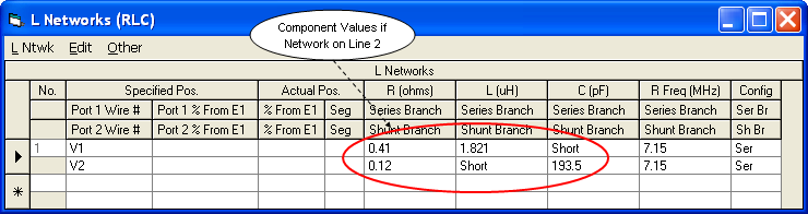
The L network type feed system is also included in the Feed2EL Excel workbook. In addition to using "real world" feedlines, the effects of component loss can also be included by specifying the capacitor and inductor Q factors. The two feedlines don't have to be 90° in length unless you want to indirectly measure the element current by measuring the voltage (perhaps with an oscilloscope) at the input end of the line as mentioned above. And you can place the network on either line 1 or line 2.
As with the "simplest" feed system it's probably not a good idea to make a decision based solely on the SWR value. Instead you might want to look at the reactance values for the L network components. For example, the screen grab at left shows the values when the L network is placed ahead of line 1 and below are the values if the network is placed ahead of line 2.
Notice that in this particular case the value of the inductor is much lower if the network is placed on line 2. |
Using EZNEC v.5 you can model the L network like this.
When creating L networks with EZNEC remember that the series branch is always entered first regardless of whether the network "faces" left or right.
Running the model and then checking the currents verifies that the network is performing as planned. Although the feedlines are both the same length (in this case 90°) the network has performed the correct voltage transformation at the input end of line 2 such that the currents at the element bases have the desired relationship.
(This EZNEC model file is included in Sample Feed2EL Models.zip.)
As was the case with the "simplest" solutions, there is a distinct difference in the F/B ratio pattern when a sweep is done over the entire 40 meter band. However, at the design frequency of 7.15 MHz the F/B ratio is exactly the same in all cases which verifies that the designs were done correctly.