In previous sections you saw how to build a model using variables and Excel formulas to control the XYZ coordinates. But in many cases you don't have to create a new model or modify an existing model; you can use a model that has straight numeric values for the coordinates yet still manipulate it as though the coordinates were set via variables and formulas.
As mentioned in the Quick Start Guide, you can move, rotate, or scale one or more wires of your model by using the Move/Copy, Rotate, or Scale buttons on the Wires sheet. (The Rotate and Scale functions also have a "copy" option.) The amount of movement, rotation, or scaling can be a fixed numeric value or can be controlled via a variable or formula.
15M Quad, move all wires
Here is an example showing how you might raise the height of a model by a variable amount; that is, change the Z axis coordinates for all wires, and control the amount of movement via a variable without the need to create any formulas.
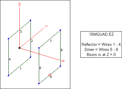
You could do this with any model. For illustration the 15MQUAD.ez model will be used. Open that model with AutoEZ.
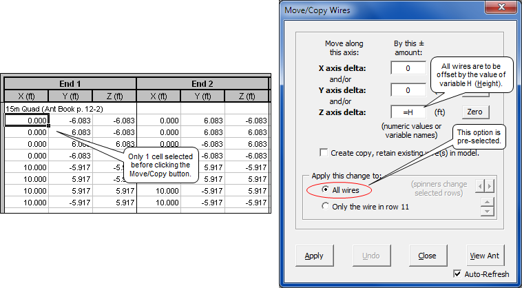
Since this is an EZNEC (.ez) type model all coordinates are set as fixed numeric values. On the Wires sheet click the Move/Copy button. In the dialog window enter "=H" (or just "H") in the Z axis delta field. Click Apply.
Important: There is nothing special about the use of H as the variable name in this example. You are free to use any valid AutoEZ variable name that seems logical to you, such as B (for boom offset) or D (for delta amount) or Z (for Z axis offset).
You'll see a reminder message informing you that the amount of movement is currently 0. To understand what that is all about click the Unhide Rows button on the Wires sheet (if necessary), which is a toggle button that switches between Hide and Unhide. Then select cell D30.
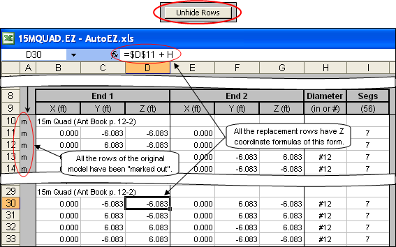
Note that rows 10-28 have been "marked" by AutoEZ with the letter "m". When a row is "marked" it means that the row (wire) will not be included in the temporary model file that is sent to EZNEC. However, the row is not deleted and can still be referenced by Excel formulas. (Rows can be marked with any letter. AutoEZ uses "m" to mean "moved along one or more axes".)
Also note that new rows have been added by AutoEZ, rows 29-47. These are duplicates of the originals except that the Z coordinates for all wires have a formula similar to what you see for cell D30. That is, the value for cell D30 will be equal to the corresponding cell of the original model (D11) but incremented by whatever the current value is for variable H. Since H hasn't been set yet it has a default value of 0 which is why the present values for cells D30 and D11 are the same. But if H had a value of, say, 10 then cell D30 would be 10 greater than cell D11. (Don't let the "$" signs in the formula confuse you. Those are used to signify absolute versus relative cell references, an Excel distinction which is not relevant to this example.)
Since you probably want to see only the "final" set of wire rows and not those which have been "marked', click the toggle button again. The button name will switch between Unhide Rows and Hide Marked Rows but notice that the formula for cell D30 does not change. As mentioned, the hidden rows can still be referenced in Excel formulas.
Now that you've seen how AutoEZ automatically builds formulas to control the wire coordinates the next step is to create a "variable sweep" setup on the left side of the Calculate sheet. For example, suppose you wanted to have the boom height range between ¼ λ and 2 λ in steps of ¼ λ. From the Variables sheet you know that ¼ λ is about 11.6 feet, so you want to sweep H from 11.6 ft (¼ λ) to 92.8 ft (2 λ) in steps of 11.6 ft (¼ λ).
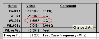
The Variables sheet shows various fractions of λ.
Important: When using the "Move/Copy" feature the variable value represents an offset or delta from the original model coordinates, not the absolute coordinate value. So in this example when you set H to 11.6 it does not mean that a wire Z coordinate will have a value of 11.6, it means that the original Z coordinate value will be incremented by 11.6.
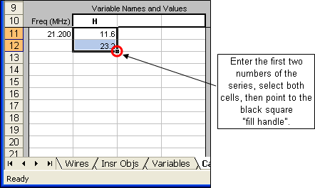
To create the sweep values you could use the Generate Test Cases button but there is an Excel trick that you might find to be more convenient. First, enter the variable name (without the "=" sign) in cell C10 of the Calculate sheet. You can use upper or lower case. Then enter the first two values of your intended sweep range, 11.6 and 23.2 in this case.
After the first two values are entered, select both cells and release the mouse button. Then point to the Excel "fill handle" which is the black square at the lower-right corner of the selection range. Press and hold the left mouse button and drag down the page.

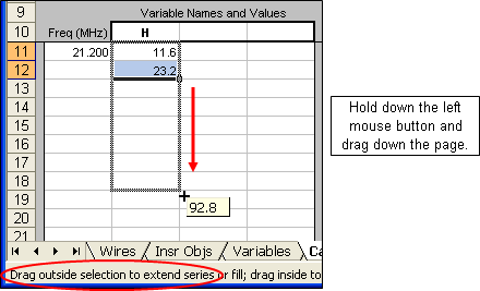
As you drag down the page the small indicator box will change. When it reaches your desired end point, release the left mouse button. Excel will automatically create a series of values using the first two numbers that you entered as the first two steps of the series.
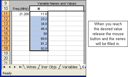
If you drag beyond the bottom of the page the window will automatically scroll down.
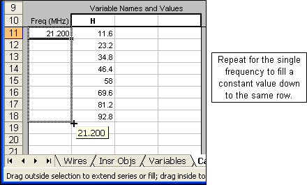
After the variable values have been set drag the fill handle for the frequency down to the same row. You may then wish to double-check that the model will change as desired by selecting any cell in the first row of the "variable sweep" range and clicking the View Ant (For Selected Row) button, then selecting any cell in the last row of the range and viewing the model again.
This may seem like a complicated process but once you become familiar with using the Excel fill handle it is very easy to create a test case setup. However, you always have the option of clicking the Generate Test Cases button. To illustrate, this is how you would generate the setup values shown above.
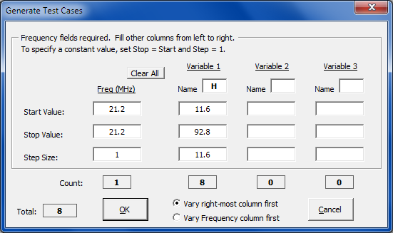
Now matter how you create the test case setup, when finished change the modeling environment to Real-Average ground, Copper wire loss, and plot type Elevation.

Then click the Calculate All Rows button. After the calculations are completed you might wish to tab to the Patterns sheet and "watch the movie" of the changing far field pattern. Notice how the number of lobes increases as the height is raised. (In the animation below you can read the value for H in the lower right corner. The outer ring has been frozen at 13.18 dBi to allow easy comparison of the patterns.)


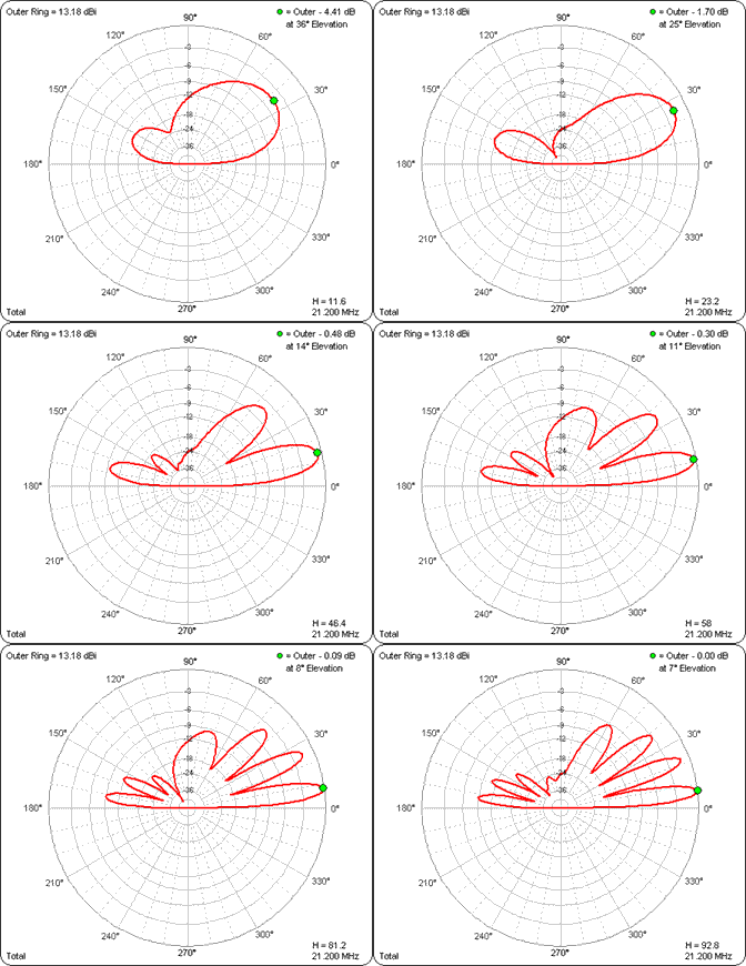
(Press Esc to stop the animations, F5 to restart.)
15M Quad, scale (some) and move (all) operations cascaded
In the above example you modified the existing all-numeric wire coordinates by using the AutoEZ Move feature. Here's a different example using "cascaded" Scale and Move operations. Suppose you wanted to experiment with changing the size of the reflector loop while leaving both the driver loop size and the spacing between the loops the same. Furthermore, you want to raise the entire antenna by 1 λ.
Important: Open the 15MQUAD.ez model again to start with a fresh copy, rather than trying to continue from the last example.
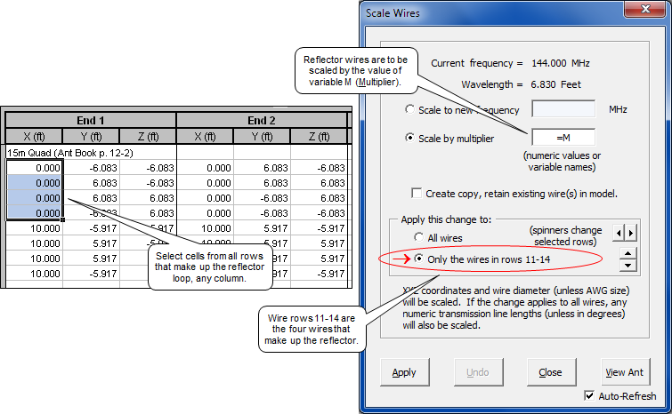
On the Wires sheet, select the four wire rows (any column) that make up the reflector. That's wires
1-4 , rows11-14 . Then click the Scale button.You can choose to scale to a new frequency in which case the scaling factor will be "Current Frequency / New Frequency" or you can scale by a specified multiplier which can be either a straight numeric value or a variable. In the dialog window first select the Scale by multiplier option then enter "=M" (or just "M") in the scale factor field. Again, there is nothing special about the variable name M. You can use any valid AutoEZ variable name.
Note that the "Only the selected wire(s)" option is pre-set, corresponding to the rows you selected before clicking the Scale button. So only a subset of the model wires will be scaled. Click Apply.
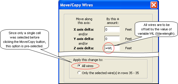
After you have done the scaling step, the second step of the "cascaded" operations is to Move (not Scale) all wires, raising them by 1 λ. From the Variables sheet you know that 1 λ is about 46.4 ft at 21.200 MHz so you could enter 46.4 as the Z axis offset. But you can also use the pre-defined variable name WL. Variable WL (or the equivalent, W) is always equal to one wavelength at the current frequency and with the current choice for units. So make sure that only a single cell is selected, click the Move/Copy button, and enter "=WL" (or just "WL") as the Z axis offset.
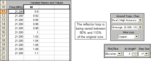
Then create a series of test cases on the Calculate sheet varying M from 0.9 to 1.1. Also, make the same changes to the modeling environment that you made for the previous example (Real-Average ground, Copper wire loss, plot type Elevation). Click the Calculate All Rows button.
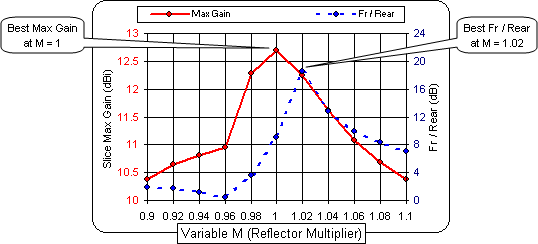
Below is one of the three pre-defined charts available on the AutoEZ Triple sheet. Note that if the reflector is made just 2% larger than the original size the Max Gain drops by less than 0.5 dBi but the
Front/Rear ratio improves by over 9 dB. (Vertical gridlines were manually adjusted for clarity in this illustration.)
Caution: When a wire is scaled, all six coordinates (
End 1 XYZ andEnd 2 XYZ) are multiplied by the same factor. Be careful when scaling loops and pay particular attention to the order of cascaded operations. For example, suppose you had done the Move step first (raising all wires by amount WL) followed by the Scale step (multiplying all coordinates of the four reflector wires by a factor of 0.9). All the X coordinates of the reflector loop are 0 so they would stay 0 after multiplying by 0.9. The Y coordinates are centered on either side of Y=0 so they would all contract by a factor of 0.9 as expected. However, because you did the Move step first the Z coordinates are now not centered on either side of Z=0. Instead, they are centered on either side of about 46.4 ft (1 λ). So when multiplied by 0.9 the loop size would contract by the correct amount but would also move down the Z axis, closer to 0. The antenna would look like this.
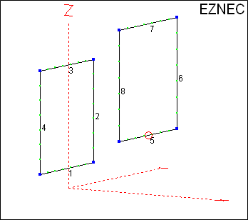
Probably not what you had in mind.