Patterns Tips and Tricks
Here are some tips for getting the most out of the Patterns sheet tab. Different topics are separated by a short horizontal bar.
You can use the Tot dB / V dB / H dB option buttons to display the Total far field space wave gain or just the Vertical or Horizontal polarization components of the far field. This is similar to clicking the Desc Options button on the EZNEC main window, selecting the Plot and Fields tabs, then choosing the "Vert, Horiz, Total" option. The difference is that with AutoEZ you see only the chosen component; with EZNEC you see all three at the same time on the EZNEC 2D Plot window.
Note that you don't have to be particularly accurate with the mouse pointer when changing options. You can click on the option button itself or on the text next to the option button.

Keep in mind that the outer ring of the AutoEZ polar plot is normally "auto-scaled" which means that it will change for each different option selection. That may fool you into thinking that the vertical and horizontal components are roughly the same magnitude with just a different shape but for most antennas that is not the case. If you want to compare magnitudes as well as shapes (as you can do with EZNEC since all three traces are shown at the same time) you can use the Freeze Now button when viewing the total field. Then when you choose the vertical or horizontal polarization component the plot outer ring will not auto-scale.
In the animation below on the left the outer ring changes from 16.10 dBi for the total field, to –17.14 dBi for the vertical component, and back to 16.10 dBi for the horizontal component. On the right the outer ring has been frozen at 16.10 dBi, making it obvious that the vertical component is much smaller than the horizontal.

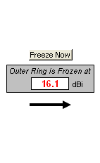
(Press Esc to stop the animations, F5 to restart/resync.)
Being able to see both a polar and rectangular view of the pattern may give you new insights into the performance of your antenna. In addition, the rectangular view allows you to quickly compare the field strength at all angles just by glancing at the horizontal (dBi) reference lines.
When viewing elevation plots over ground, that is, when the pattern range is 180 degrees, the rectangular view will always start at 0° elevation angle as the left vertical gridline and show the 180° elevation angle as the right vertical gridline. You can correlate the polar and rectangular patterns by noting the position of the green marker dot.
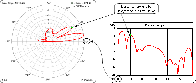
Note that there is no space wave far field radiation at 0° or 180° elevation. EZNEC reports these values as
-99.99 dBi . Rather than plot these meaningless numbers you can choose a Low Clip limit for the rectangular view, set at-40 dBi above.For azimuth plots (or Free Space elevation plots), when the pattern range is 360 degrees, you can choose the Start Angle to be used for the left vertical gridline. You may wish to align the rectangular view such that the forward lobes of the pattern fill the left half of the chart and the back lobes fill the right half (below, right top). Or you might want to center the main forward lobe in the center of the chart (below, right bottom). In the illustration below both rectangular charts show the same information, the top with a start angle of 270° and the bottom with a start angle of 180°
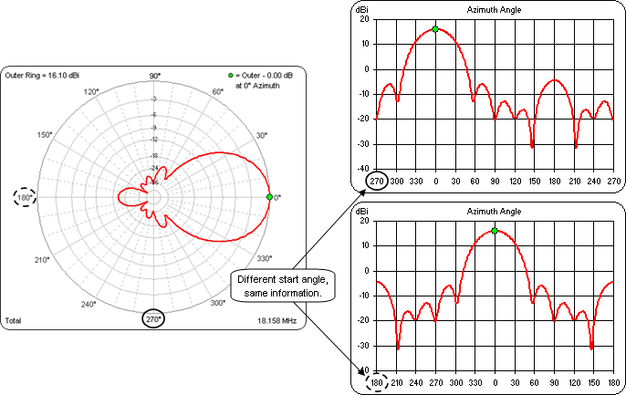
If you leave the Start Angle at "Auto" then AutoEZ will assign a value that is 90° "before" the direction of the main lobe, like the top example above. That way the forward lobes will fill the left half of the chart regardless of whether you have defined the antenna elements to be aligned with the X axis (main lobe points up or down) or the Y axis (main lobe points right or left).
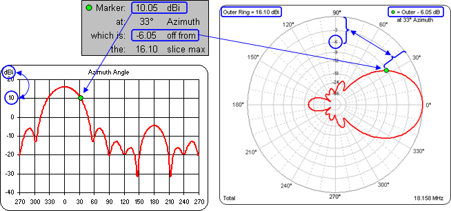
Keep in mind that the rectangular view shows dBi whereas the polar view shows "dB down" from whatever the dBi value is for the outer ring. The rectangular view horizontal gridlines (dBi) are not the same as the polar view circular gridlines (dB down).
In the illustration below the marker has been placed at 33° azimuth angle. At that angle the field strength is 10.05 dBi, just slightly above the "10" horizontal gridline on the rectangular view. The same field strength is also 6.05 dB less than the 16.10 dBi outer ring setting, just slightly below the
"-6" circular gridline on the polar view.
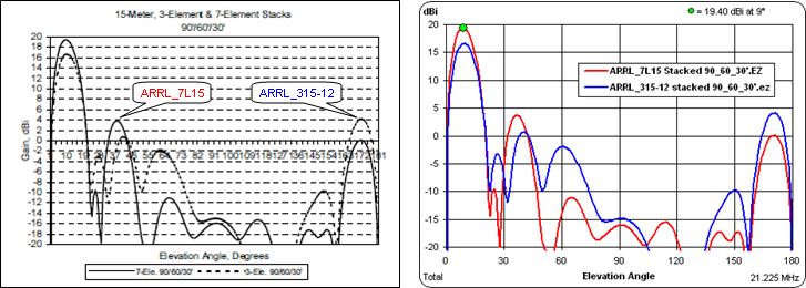
If you have a recent copy of The ARRL Antenna Book you may have seen rectangular patterns in that publication. For example, below on the left is Fig 36 from Chapter 11 of the 20th and 21st editions. It shows the elevation pattern for two different stacks of Yagis, 7 elements stacked at 90/60/30 ft and 3 elements stacked at 90/60/30 ft. On the right are the same patterns in AutoEZ, created by opening and calculating the "ARRL_315-12" model, taking a snapshot, then opening and calculating the "ARRL_7L15" model.
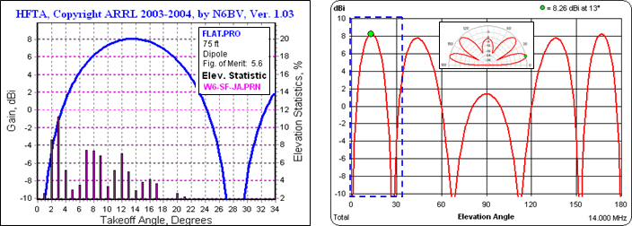
The Antenna Book also has numerous examples taken from the HFTA program by N6BV. These too show rectangular elevation patterns, along with propagation statistics displayed on a secondary vertical scale. Note that the HFTA patterns stop at 20, 25, or 34 degrees elevation angle and many of the Antenna Book examples use a Low Clip limit of 0 dBi. Hence the elevation pattern shown by HFTA is a subset of what AutoEZ shows but allows a much better comparison with the propagation statistics.
Below on the left is the pattern from HFTA for a 14 MHz generic dipole at 75 ft along with the propagation statistics for the path from Northern California to Japan and the Far East. On the right is the AutoEZ pattern for the EZNEC model BYDIPOLE.EZ, raised to a height of 75 ft. The blue dashed box shows the portion of the elevation pattern that is common to both programs.
Although the example above used flat ground (FLAT.PRO), keep in mind that HFTA is specifically designed to create elevation patterns using generic antenna models over irregular terrain. EZNEC and other modeling programs can produce field strength patterns for very specific antenna models but only over flat terrain.
As mentioned, you can use the green dot marker as a way to help correlate the polar and rectangular views. And of course you can use the marker to explore pattern variations even if you focus only on a single view.
There are several ways to move the position of the marker.
While manipulating the marker, if you happen to double-click on the trace the marker will move to the correct new position but you will also see an Excel "Format" dialog window. (The exact title of the dialog may vary.) If that happens just press the Esc key twice to clear the dialog and return to normal operation.
- You can click on the primary (red) trace of either the polar or rectangular chart. The angle of the marker (elevation or azimuth) will stay "in sync" between the two views.
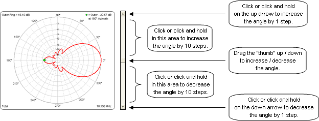
- Using the scroll bar you can drag the box, also called the "thumb", to change the angle of the marker.
- You can click on the up arrow at the top of the scroll bar to increase the angle by 1 step, which is usually 1° if you chose a 1° plot Step Size on the Calculate sheet. If you click and hold on the up arrow the angle will continue to increase by 1 step. The down arrow at the bottom of the scroll bar works the same way to decrease the angle.
- If you click or click and hold on the portion of the scroll bar between the thumb and the up arrow, the angle will increase by 10 steps. Click on the portion of the scroll bar between the thumb and the down arrow to decrease the angle by 10 steps.
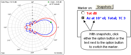
- If you have one or more snapshots showing you can switch the marker by clicking on the snapshot trace.
- You can also switch the marker by clicking on the appropriate option button or by clicking on the text next to the option button. When you switch the marker using this method the angle will not change as the marker moves between traces, which may be difficult to do if you click directly on the trace.

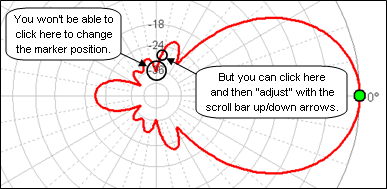
If you try to click on a portion of the trace that is "underneath" one of the circular gridline labels
(-3, -6, -9, etc) the marker will not move. However, you can click on a "close by" spot and then use the scroll bar up/down arrows to move the marker to the desired position.
You can use the Snapshots button to compare patterns between different test cases for the same model, as shown in some of the examples above (red primary trace vs blue snapshot trace). Since snapshots persist until they are manually erased you can also use this feature to compare patterns from different models. That is, open and calculate model A, take a snapshot, then open and calculate model B.
If you would like to make a permanent copy of a trace you can click Snapshots and then Save Primary Trace to File. At some later time you can then use the Recall Trace to Snap Position button to show the trace.
Finally, although seldom used, you can display any EZNEC 2D trace file (file types .PF and .P#) on the AutoEZ Patterns sheet. On the EZNEC 2D Plot window select File > Save Trace As to save a trace file. Then with AutoEZ click Snapshots and then Recall Trace to Snap Position. Navigate to the folder where you saved the EZNEC trace file and open that file. It is probably more convenient to just open the EZNEC model (.ez) and calculate. However, if you have a collection of EZNEC trace files this is a way to show both a polar and rectangular view.
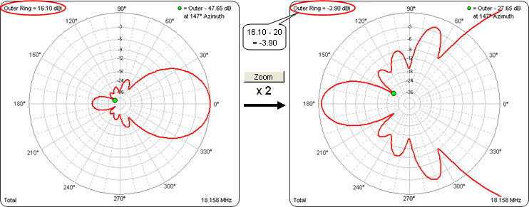
To resolve fine details for deep nulls on the polar view you can use the Zoom button. Each click will subtract 10 dBi from the outer ring setting. Click a total of 4 times to "unfreeze" the outer ring and return to normal operation.
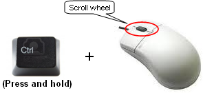
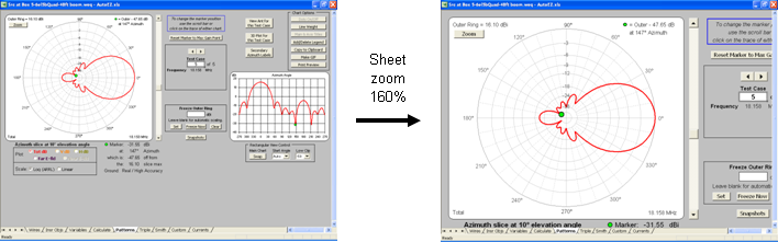
On the other hand, if you want to magnify the entire chart you can take advantage of the Excel "sheet zoom" feature. Press and hold the Ctrl key while rotating the mouse scroll wheel. Each forward or backward click of the wheel will increase or decrease the magnification of the current sheet tab by 15%.
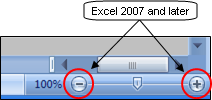
With Excel 2007 and later you can use the mouse scroll wheel, as above, or you can use the zoom controls in the status bar at the bottom of the window. Each click on the "+" or "–" button will increase or decrease the magnification of the current sheet tab by 10%.
Using one or the other of these methods you can make the main chart fill the entire window.
Electric Field Strength - Far Field
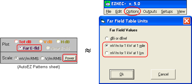
You can use the Far E-fld option button to display the field strength in mV/m or V/m rather than dBi. This is similar to clicking the Options menu on the EZNEC main window, then Far Field Table Units, then selecting either of the mV/m options. (Note that this changes only the EZNEC Far Field Table, not the EZNEC 2D Plot.) However, with AutoEZ you can choose a specific power level and a specific distance.
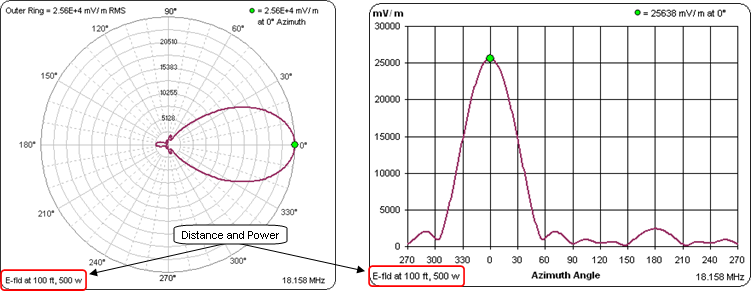
The distance and power for the Far E-fld are shown in the lower-left corner of each (full size) chart. Note that the circular gridlines on the polar chart will have rather arbitrary values. You may find it easier to use the rectangular view. Also, the rectangular view will always show mV/m even if you choose V/m for the polar view.
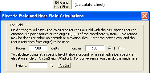
The Power button can be used to change the power level without the need to rerun the calculations. If you want to change the distance use the E-fld and Near Field button on the Calculate sheet.
If you change the power or distance via the above dialog it will be necessary to rerun the calculations.
Electric or Magnetic Field Strength - Near Field
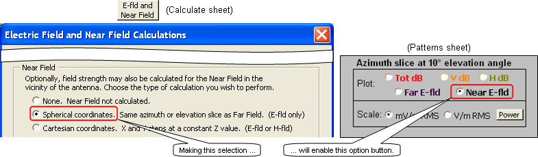
To do Near Field analysis you also use the E-fld and Near Field button on the Calculate sheet. You can choose either Spherical or Cartesian coordinates. This choice affects both the way the points in space where the field strength will be calculated are defined and the way the results will be displayed.
If you choose Spherical coordinates the Near E-fld values will be calculated for the same azimuth or elevation slice as is used for the Far Field data.
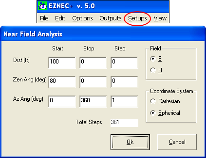
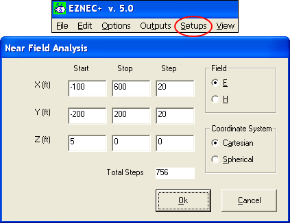
This is equivalent to clicking the Setups menu on the EZNEC main window, then Near Field, then making entries in the EZNEC dialog as shown below. Note that when using the EZNEC dialog you specify the zenith angle instead of the elevation angle. (The EZNEC dialog is shown just for comparison. AutoEZ will handle all of this under the covers.)
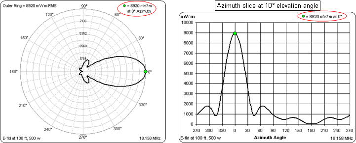
The calculated values will be displayed using the polar and rectangular charts on the Patterns sheet tab.
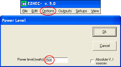
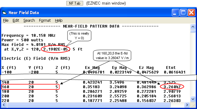
To correlate the patterns shown by AutoEZ with the raw data calculated by EZNEC you must first click the Options menu on the EZNEC main window, then Power Level, then enter the power level that was specified for AutoEZ.
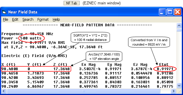
After that is done click the "NF Tab" button on the EZNEC main window. EZNEC always shows Near Field data in Cartesian coordinates even if the points in space were specified using Spherical coordinates. A bit of trigonometry will convert the X/Y/Z coordinates shown in the EZNEC Near Field Table to the radius and elevation angle that were used by AutoEZ.
Instead of Spherical you can use Cartesian coordinates to define the points in space. You specify an X/Y grid of points at a constant Z (height) value. When Cartesian coordinates are used you can also choose between E-fld and H-fld.
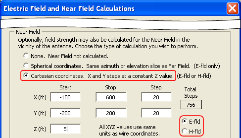
This is equivalent to making entries in the EZNEC "Near Field Analysis" dialog as shown below. (Again, the EZNEC dialog is shown just for comparison. AutoEZ will specify all of this when building the model to be sent to EZNEC.)
After the calculations have been done a new sheet tab, NF 3D, will be available.
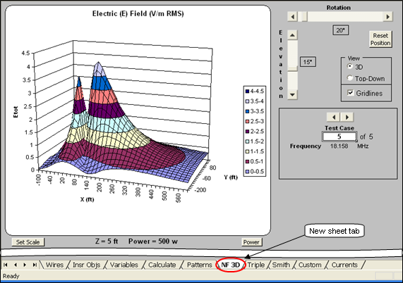
You can use the Rotation and Elevation scroll bars to change the viewing perspective for the 3D chart. The animation below shows the chart being rotated in 30° steps.
(Press Esc to stop the animation, F5 to restart.)The 3D chart gives a decent visualization of the points in space but there's no way to determine exact data values. For that you'll need to refer to the EZNEC Near Field Table. To correlate the EZNEC table with the chart you might wish to show the Top-Down view.
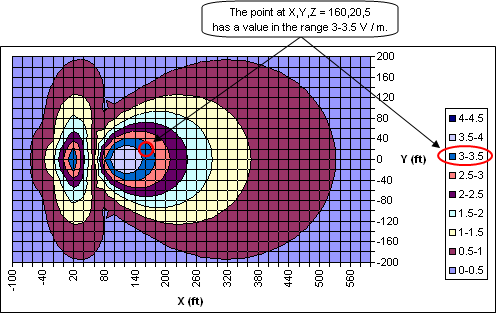
The point circled on the chart above can be found by scrolling down in the table to the appropriate
X,Y,Z coordinate row.
When working with Near Field data keep these two points in mind, quoted from the EZNEC Help:
"Note that 'Near Field' analysis actually reports the total field, so it's valid at any distance, including far from the antenna. It can also be used in the standard EZNEC program for evaluating the ground wave."And especially this:
As of this writing, EZNEC and similar programs are accepted by the FCC and some counterpart bodies in other countries as permissible for calculating compliance with RF exposure requirements. However, EZNEC results should never be used in any judgements regarding human safety. Please carefully read the Legal Disclaimer for further information.
Using 2 Ground Media
Selecting the Use 2 Media option on the Calculate sheet lets you include a second ground medium in the model.
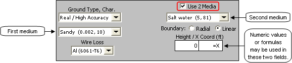
Use of two media is covered in the EZNEC Help sections "Real Ground Types", "Ground Media - Using Two", and "Media Window - Using". The following is an edited compilation of that information.
When using either of the Real ground types the ground may be broken into two "media", each having its own conductivity and dielectric constant. The second medium can be at a different height but must be at the same level or below the first medium (which is always at height 0). The two media can be arranged in concentric rings (radial boundary) or parallel slices (linear boundary).Note that you may use formulas in the height and boundary fields. In the illustration above a numeric constant ("0") is used for height and a formula ("=X") is used for the linear boundary X coordinate. Any variable name will do, it need not be X.If the boundary type is radial the first medium is a disk with the specified radius; the second medium occupies the remainder of the (infinite) ground plane at a height at or below the first medium. If the boundary type is linear the first medium occupies the ground to the left (toward the negative side) of a line parallel to the Y axis and with the specified X coordinate; the second medium occupies the remainder of the (infinite) ground plane at a height at or below the first medium.
A very important thing to understand is that the second medium is used only for far field pattern calculations and is ignored for all other purposes including impedance and SWR calculations. Be careful when using two media and keep the following in mind:
1. Even if you place the antenna over the second medium, EZNEC will always use the ground constants and height (Z = 0) of the first medium for calculation of the impedances and currents.When Real/High Accuracy ground is chosen, the constants of the first medium are used during determination of antenna impedance and currents. When Real/MININEC ground is chosen, Perfect ground is used during determination of antenna impedance and currents. For either Real ground type, the constants of both media are used during pattern calculation by modifying the strength and phase of the field reflected from the ground.2. The second medium is used only for far field calculations. Near Field and Ground Wave calculations assume that the first medium is of infinite extent; the second medium is ignored.
3. The effect of the second medium is taken into account only in a very simplified way. The vertical pattern is generated by tracing "rays" direct from the antenna and reflected from the ground. When a second medium is used, the ground reflection "ray" is determined by whichever medium it strikes the top of. The "ray" does not penetrate either medium and diffraction or similar effects aren't considered. Because of this, a highly conductive inner medium and normally conductive outer medium is not a good model of a ground radial system, and shouldn't be used for this purpose.
4. Buried wires in EZNEC Pro/4 will always be treated as though they're immersed wholly in the first medium.
Using a formula allows you to create a "variable sweep" set of test cases. Here is how the far field elevation pattern for a 20m quarter-wave vertical changes as the X coordinate of the linear boundary is varied, with sandy ground on the left and salt water X feet from the antenna on the right. The X coordinate value (distance to water) is shown in the lower right for each frame of the animation.
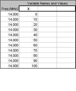
(Press Esc to stop the animation, F5 to restart.)