Contents
- Overview; Supported Hardware/Software
- Description of Buttons
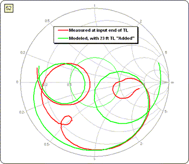
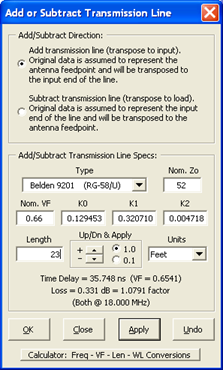
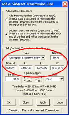
- "Add Transmission Line" Feature
- "Subtract Transmission Line" Feature
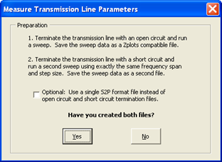
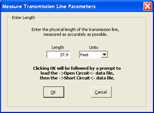
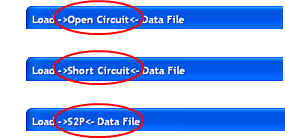
- "Measure Transmission Line Parameters" Feature
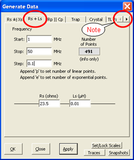
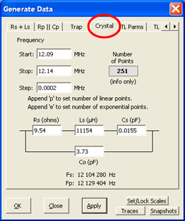
- "Generate Data" for Impedance Data Feature
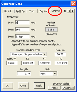
- "Generate Data" for Transmission Line Parameters Feature
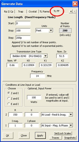
- "Generate Data" for a Transmission Line at Fixed Frequency Feature
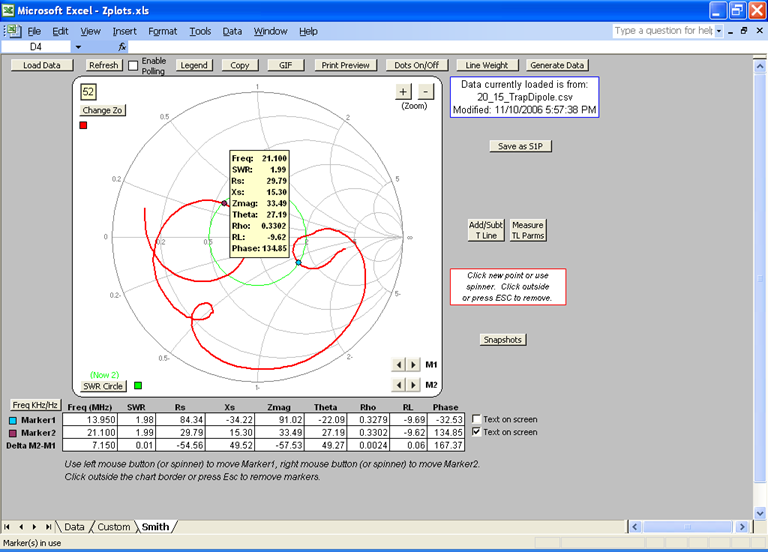
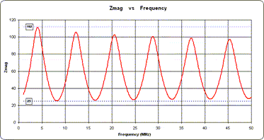
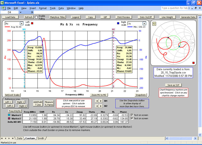
- Numerical Values for Plotted Points: Chart Tips, Markers
- Trace Line Colors
- Download and Prerequisites
- What is ZplotsLink? (VNWA Users Only)
- Manual Entry of Data for Display with Zplots
- Remote Control of the AIM and/or VNWA Devices
- Change History
- Appendices (each opens in a separate window)
- Antenna Measurements via a Feedline
- Seeing the Effects of Phasing Lines
- Resolving the Sign of X (applies only to VNA1 and miniVNA)

This web page contains dozens of images. If they don't all load you may see a red X as a placeholder. Try pressing the "Refresh" key on your browser. Poking the red X with a stick generally does not help.
Zplots is an Excel application that allows you to plot impedance and related data obtained from a variety of sources. You can plot on both an XY chart and a Smith chart as well as view the data in tabular format.
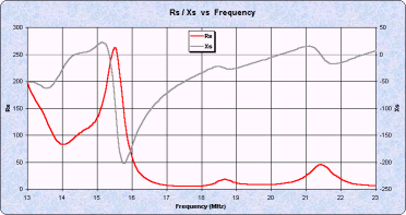
The XY chart can be customized with your choice of trace lines. Frequency (in MHz) is always shown on the X axis. On the primary (left side) or secondary (right side) Y axis you can plot:
Note concerning RL: Return loss is of course a positive number. In Zplots it is plotted as a negative number merely as a convenient way to show a reverse scale, with zero at the top and higher (magnitude) values lower down. This is the typical way of plotting RL.
- SWR - Standing Wave Ratio
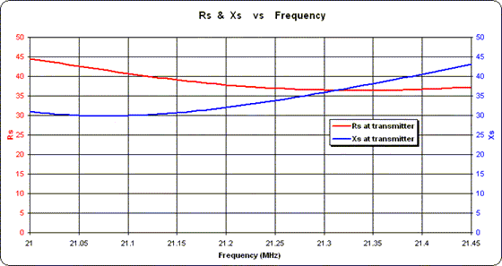
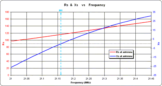
- Rs - Resistance, series form
- Xs - Reactance, series form
- Zmag - Impedance magnitude
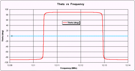
- Theta (deg) - Impedance angle
- Rho (mag) - Reflection coefficient magnitude
- RL (dB) - Return Loss, plotted as a negative number to show "reverse" scale (see note below)
- Phase (deg) - Reflection coefficient angle
- % Reflected Power
- Q - Quality factor, |Xs| / Rs
- Rp - Resistance, parallel form
- Xp - Reactance, parallel form
- Ls (µH) - Equivalent inductance for series Xs, both positive and negative
- Cs (pF) - Equivalent capacitance for series Xs, both positive and negative
- Lp (µH) - Equivalent inductance for parallel Xp, both positive and negative
- Cp (pF) - Equivalent capacitance for parallel Xp, both positive and negative
Negative values for Ls, Cs, Lp, and Cp may be interpreted to mean the amount of inductance or capacitance which must be added, in series or parallel respectively, to "cancel out" the corresponding reactance.
The order of the items in the above list has no special significance other than that the items most likely to be chosen for plotting are near the top. On the secondary (right side) Y axis you can also choose "(none)" to indicate no secondary plot line.
A Mini-Smith chart is shown on the same sheet with the XY chart. To see both the XY chart and the Mini-Smith at the same time you must have your screen resolution set to 1024x768 or higher and you must maximize both the Excel window and the workbook sub-window (using the lower set of size buttons). Alternatively, on the Excel menu you can select View | Zoom and choose a magnification level less than 100%.
Zplots can read impedance data from:
- AIM - Antenna Analyzer AIM430 / AIM4160 / AIM4170 by W5BIG (more info) / (forum)
On the menu bar select File | Save Graph. The current scan will be saved in two formats. The *.scn file is used by AIM if you want to reload the scan data at a future time. AIM also saves the scan data in *.csv format that can be read by Zplots. Software must be version 547 or later.
- VNA2180 - Vector Network Analyzer by W5BIG (more info) / (forum)
On the menu bar select File | Save Port A Graph. The *.csv saved file can be read by Zplots. Note that only the Port A file format is supported. Zplots will not recognize the Port B format file.
- VNA4Win - Windows software for the N2PK VNA by GM4PMK and GM3SEK (more info) / (forum)
After at least one sweep has been completed, the Save Data button will appear when the sweep is stopped. Clicking Save Data opens a dialog box to allow you to save the measurement results as a *.csv file. Zplots can read this file.
- Exeter - VNA Control Software by W8WWV (more info) / (forum)
An Exeter data set is created whenever a data capture finishes without error. You may then use the Save As button (or File | Save Data Set As on the menu bar) to save the data in *.csv format. Zplots can read this file. Note that Zplots makes use of only the default fields in the file. The file may contain other fields as well; these are ignored by Zplots.
- Refl.exe/Trans.exe/GrpDel.exe - DOS store data programs by N2PK (more info) / (forum)
These programs can create various .DAT files and Zplots can read these files. If the file contains multiple DUT data sets you will be asked which one you wish to show. Note that it is not necessary to change the file extension to something other than .DAT, although you may do so for other reasons.
- myVNA - GUI program for the N2PK VNA by G8KBB (more info) / (forum)
Use "Load & Store Data" and then "Save to File". In the "Save as type" drop down list select "CSV Data Set" -or- "VNA4Win CSV files" -or- "Touchstone Format". For Touchstone Format, be sure you have already used "Set Touchstone File Options" and selected 'S' as the "Save Parameter Type". You may choose any option for "Save Format".
- VNA1 / miniVNA / IG miniVNA / miniVNA PRO / vna-J / Blue VNA -
Antenna Analyzer and miniVNA by IW3HEV, et al. (more info) / (forum)
- VNA1: Save sweep data in *.csv format via File | Save As on the menu bar. Software must be version 1.1.8 or later.
- miniVNA: Save sweep data in *.csv format via File | Save As (.csv) on the menu bar. When prompted to "Select csv Format" be sure to use a comma as the data separator. Software must be version 2.2.8 or later.
- IG miniVNA: Save sweep data in *.csv format via File | Save .CSV for Zplots on the menu bar.
- miniVNA PRO: Use File | Export .csv (Zplots) -or- select the
"S-parameters" tab and then follow the procedure for creating either 1-port or 2-portS-parameter files. Software must be version 2.4.0.4 or later.
- vna/J: Use Export on the menu line (or the corresponding toolbar button) to export the scan data in "Zplots" format -or-
"S-parameter" format. The DL2SBA vna/J software supports both the original miniVNA and the miniVNA PRO hardware. Software must be version 2.6.4 or later. (more info)
- Blue VNA: This is an Android only application by YO3GGX to control Bluetooth enabled antenna analyzers or VNAs. Supported devices are miniVNA (equipped with a Bluetooth add-on) and miniVNA Pro (with or without the Extender). See "Exporting data to be used in external applications" in the user guide. (more info)
- TAPR VNA - TAPR Vector Network Analyzer (more info) / (forum)
Use File | Export on the menu bar and then choose Rectangular or Polar format (but not csv format).
- DG8SAQ VNWA - DG8SAQ Vector Network Analyzer (more info) / (forum)
If you have made one-port measurements (such as for an antenna system), on the menu bar use File | Export Data | Trace | S11 and then choose any of the three options to create a file in s1p format. If you have made two-port measurements (such as for a filter), on the menu bar use File | Export Data | S2P and then choose any of the three options to create a file in s2p format.
As an alternative to File | Export Data, you may enable an external tool in the VNWA Tools | Configure Tools dialog panel and check the "Autowrite measurement data" box. If this box is checked (and the tool is enabled), VNWA will automatically write file 'default.s2p' to the folder specified in "Path" for that tool after each scan is completed. Zplots can read this file. (This feature available in VNWA version Beta 33.f and later.)
- RigExpert (all models) - with AntScope software (more info) / (forum)
On the AntScope menu bar choose File | Export to | CSV file or File | Export to | Touchstone file. Zplots can read either of these files.
- SARK-110 / SARK-100 - Antenna Analyzers by EA4FRB (more info)
For the SARK-110 see "Saving and Recalling Measurements" in the SARK-110 User's Manual. For the older SARK-100 see "PC Software" in the SARK-100 User Manual.
- DL1SNG FA-VA - DL1SNG FA-VA Antenna Analyzer (more info)
The DL1SNG application software for the PC can create a *.csv file containing impedance values in real and imaginary format. Zplots can read this file.
- Touchstone s1p/s2p Generic (more info) / (specs)
Zplots can read Touchstone s1p/s2p format files that are produced by many different applications, with the following restrictions and limitations:
- Only one-port (s1p) and two-port (s2p) type files are supported. The file name must include the extension .s1p or .s2p.
- Data type S only, not Y, Z, H, or G.
- "Keywords" as described in Version 2.0 of the Touchstone File Format Specification are not allowed.
For s1p files, Zplots will assume that the file contains S11 (reflection) type data. This is the Touchstone standard, although some programs such as the DG8SAQ software mentioned above can create s1p format files containing non-S11 data. Such files can be read by Zplots although the results may be confusing.
For s2p files, Zplots can display various subsets of the s2p data: Reflection (S11 or S22) only, Transmission (S21 or S12) only, or both (S11/S21 or S22/S12), for either the Forward or Reverse direction. If Reflection data is displayed, with or without Transmission data, then a Smith chart is also shown. To change the subset selection use the "Change S2P Subset(s)" button (see below).
Unlike many VNA control programs and other software that can read Touchstone s2p files, Zplots cannot display both forward and reverse data at the same time. However, you can display one type of data, take a Snapshot of the trace(s), and then display another type of data. (See below for more details about Snapshots.)
- EZNEC - EZNEC Antenna Software by W7EL (more info)
Every time you run either an SWR sweep using the SWR button or a Frequency Sweep via Setups | Frequency Sweep on the menu bar, EZNEC will automatically create a file named LastZ.txt. With EZNEC v. 5.0 the file is written to the EZNEC home folder, typically
C:\Program Files\EZW. With EZNEC v. 6.0 the file is written to the folder specified under Options | Folders | Output Files, typically sub-folder"EZNEC 6.0" under"My Documents" . Zplots can read the LastZ.txt file.Because EZNEC overwrites this file every time a sweep is done you may have decided to make a copy under a different name. You may also have changed the file extension from .txt to .csv to allow more convenient use with a spreadsheet program. Zplots can read the file no matter what name or extension it may have.
Caution for EZNEC v. 5.0 under Vista / Windows 7 / Windows 8 / Windows 10: If you have installed EZNEC v. 5.0 to the default location, under these operating systems the LastZ.txt file will probably be written to folder
C:\Users\[UserName]\AppData\Local\VirtualStore\Program Files (x86)\EZW. You must navigate to that folder when attempting to load the file.- Antenna Model - Software for the Analysis of Wire Antennas by Teri Software (more info)
After you have done a scan via Calculate | Frequency Scan on the menu bar you will have the option to save the impedance data (and other data) for the model. On the menu bar choose File | Export Impedance Data Points, or press Ctrl-M. A file named
[model]Impedances.csv will be written to the Archive folder. (If you want the file to go someplace else press Shift-Ctrl-M instead of Ctrl-M and you will get a Save As dialog box.) Zplots can read this file. Software must be version 635 or later.Some of the programs mentioned above can create "Transmission" and/or "Group Delay" type data as well as "Reflection" data, either as a separate file or as part of a Touchstone s2p file. Zplots can read this data and show an XY plot for:
When a "Transmission" or "Group Delay" type data is used as input to Zplots the Smith charts and certain other program functions will be disabled.
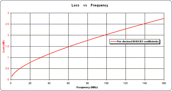
- TL (mag) - Transmission loss (also called insertion loss) magnitude
- TL (dB) - Transmission loss in dB, plotted as a negative number to simulate "reverse scale"
- Phase (deg) or Grp Delay (µsec) - Phase shift or Group delay, depending on file contents