Examples of using AutoEZ have been created from time to time to address questions raised on various forums and reflectors. This is a collection of such examples, in some cases slightly edited. Step by step instructions are omitted to maintain brevity.
Spiderbeams with Variables
In response to a question about tuning a commercial Spiderbeam antenna I built a couple of models, one 5-band and one 3-band, in which all the dimensions are controlled via variables and formulas. Hence a) you can easily adjust the lengths of the driven elements to put the SWR minimums where you want them, b) you can experiment with the other element lengths and boom positions to see the effect on the patterns, and c) if you have a homebrew antenna you can adjust the model to match what you built.
Segment length tapering is used in the models, with very short segments at the element centers where the currents are highest and where (on the drivers) the source and transmission lines are connected. Longer segment lengths are used at the outer ends of the elements. This results in very good Average Gain Test values, and hence very good model accuracy, while still keeping the total number of segments down for faster calculation times.
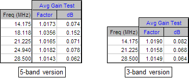
In terms of the absolute value of the Average Gain Test dB level, the LB Cebik guidelines are:
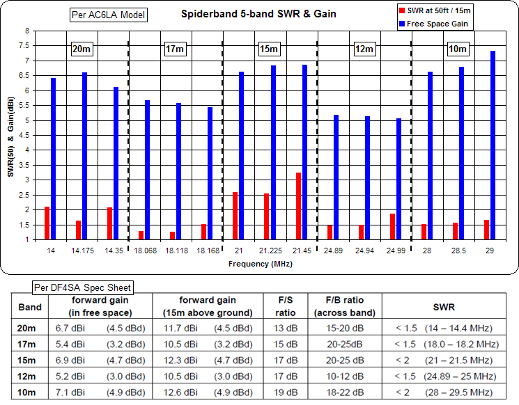
|AGT| < 0.2 dB: "Model is considered to have passed the test and is likely to be highly accurate."Below are the modeled results for SWR and Gain for the 5-band version at three frequencies in each band. The table below the chart is from the Spiderbeam spec sheet
|AGT| > 0.2 dB: "Model is quite usable for most purposes."
|AGT| > 0.4 dB: "Model may be useful, but adequacy can be improved."
|AGT| > 0.8 dB: "Model is subject to question and should be refined."(link) . Pretty good correlation for Gain but for SWR the model is a bit more pessimistic.
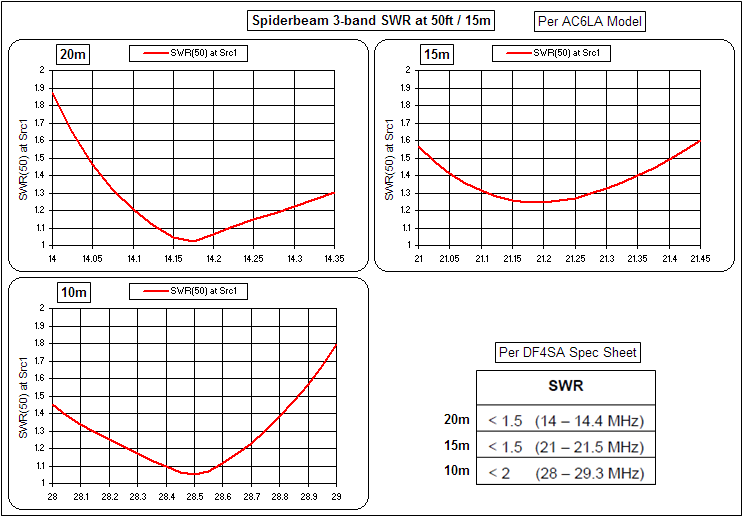
And here are the full SWR curves for the 3-band version. These are more in line with the 3-band specs.
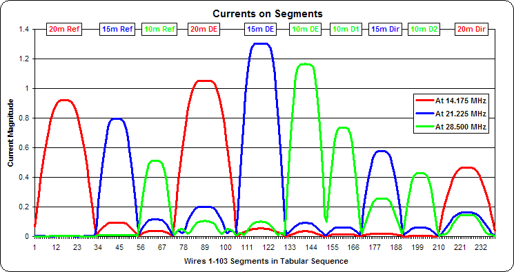
Here's another way of looking at the 3-band version. This chart shows the currents on all wires at three different frequencies. For example, the red trace shows that at 14.175 MHz most of the current is distributed across the 20m reflector, 20m driven element, and 20m director. There is very little current on the 15m and 10m elements. At 28.5 MHz (green trace) the situation is not quite as clean, with the 15m director taking some of the action that was intended for the two 10m directors.
All the dimensions in the models were copied from the Spiderbeam Construction Guide v. 2.20 (available by request here) and then the AutoEZ optimizer was used to fine-tune the driven element lengths. Note that the commercial version of the Spiderbeam uses Wireman CQ-532 copper-clad steel wire
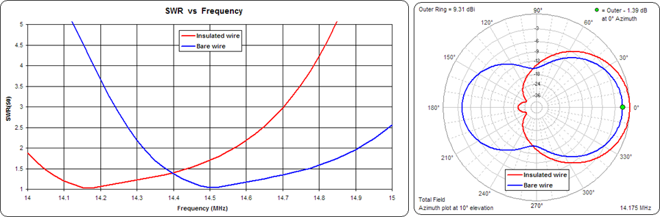
(link) , 0.0445" diameter with a 0.020" polyethylene insulation (assumed dielectric constant 2.26). The models reflect that.If you use bare wire without changing the element dimensions these are the kind of differences you'll see. This is for the 3-band model on 20 meters.
Models:
Unzip and save to your computer then use the Open Model File button from within AutoEZ.
The G3TXQ Cobweb
Steve Hunt, G3TXQ, developed a variation of the commercial 5-band CobWebb antenna by G3TPW and has a nice
web page describing his version. I decided to develop a model in which everything is controlled via variables to see how close I could get to the actual measurement specs as shown on Steve's page. Dimensions below are in inches.
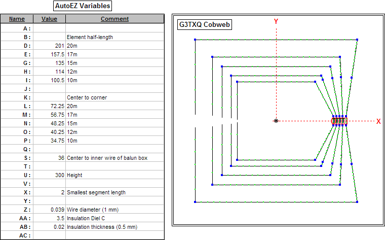
The variables for the element half lengths (D through I), for the center to corner distances (L through P), and for the center to balun box distance (S) are all inter-connected. That is, if you increase D (20m half length) the 20m element tips will move closer to the X axis. If you increase L (20m center to corner) the entire 20m square will get larger and the element tips will move away from the X axis. If you change S (center to balun) the tips will move closer or farther away depending on what it takes to keep D the same.
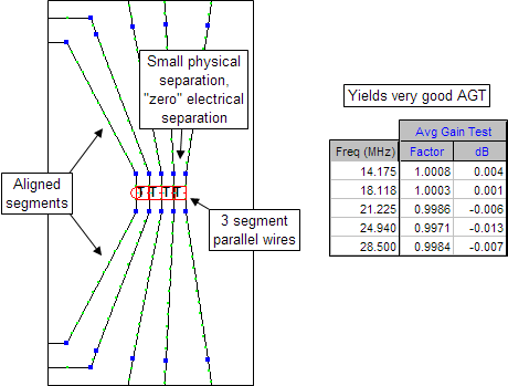
To improve the accuracy of the model I used a trick developed several years ago by LB Cebik. The feedpoints for the elements are physically separated by a small amount at the centers but are electrically joined by "zero" length (almost) and zero loss NEC transmission lines. Making the connection between elements this way, as opposed to having the elements physically connected to a common center wire, results in much better Average Gain Test results, hence more reliable impedance and gain values. For more information on the use of "zero" length transmission lines see here.
Another trick to improve model accuracy is to make sure that segment junctions are aligned, particularly important at high current regions. Here's an exploded view of the feedpoints.
With all that out of the way it was time to tune the elements for resonance.
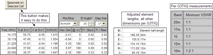
Finally, I ran a sweep from 14 to 30 MHz to compare with Steve's measurements.
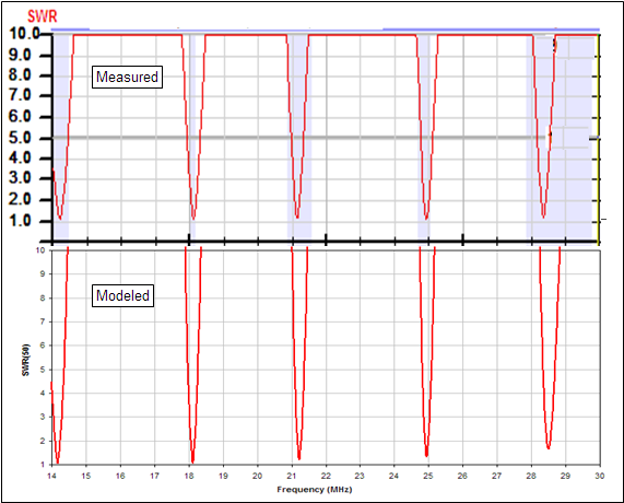
Not bad. I couldn't quite get the minimum SWRs on 12m and 10m that Steve got but otherwise the model and the measurement are remarkable close.
Steve also had this to say:
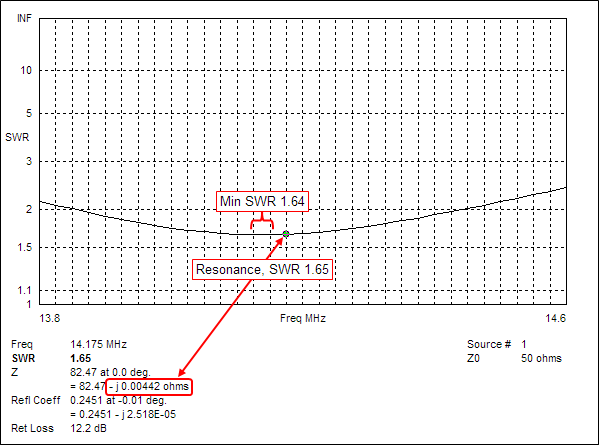
One other interesting feature of the cobweb I forgot to mention: try plotting its resonant frequency - say for the 20m band - at varying heights above ground, and compare that with a linear dipole.To do this with EZNEC typically the first step would be to run a frequency sweep and look at the SWR plot to find the minimum |X| frequency (resonance). That will not necessarily be the same as the minimum SWR. You'd probably want to include out-of-band frequencies to make sure you don't miss the dip. For a 20m antenna that might be 13.8 to 14.6 MHz and the plot might look like this.
Make a note of the frequency, change the height of the model, and repeat. Then manually create a plot of resonant frequency vs height.
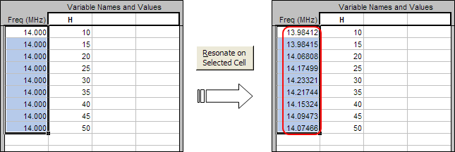
With AutoEZ the process is easier. If "H" is the variable that controls the height of your model in feet, and you want to find the resonant frequency when "H" ranges from 10 to 50 feet, set up a series of test cases all at the same initial frequency but at different heights. Then select all the frequency cells and click the Resonate button.
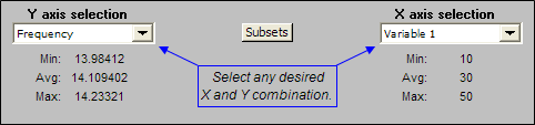
You can then tab to the Custom plot sheet and plot "Frequency" on the Y axis vs "Variable 1" (which is the height in feet) on the X axis.
So I did just that with the G3TXQ cobweb which had the 20m element already length-adjusted to be resonant at 14.175 MHz when the antenna is at 25 feet. Then I did a simple dipole which was also length-adjusted to be resonant at 25 feet, using the same wire size, wire insulation, and ground type as the cobweb. For both I did the calculations up to 70 feet, about 1 wavelength on 20m.
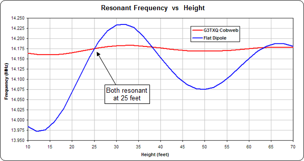
For the dipole, if you trimmed for the correct length when the antenna was only 10 ft off the ground you'd be in for a rude surprise when you raised it to 30 ft. Not so for the cobweb.
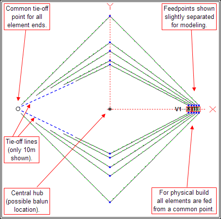
Here's a different variation; a diamond shape with separate element feedpoints (like a hexbeam) as opposed to "ganged" feedpoints.
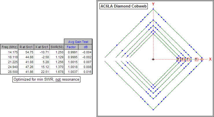
The extra wire junctions (small blue squares near the corners) in the image above are just to keep the segment boundaries aligned for more accurate modeling. In actual construction each half-element is continuous from feedpoint to tip. And note that the element overall lengths (from east side feedpoint to west side tip) were optimized for minimum SWR, not for resonance.
The advantage of this design is that no separate support is needed for the balun box. The disadvantage is that you must construct four short "quad 50 ohm" 12.5 ohm interconnect transmission lines (Steve's idea).
The 4:1 balun / main feedline connection is at the outermost (20m) element. The interconnect lines could be dressed along the top of the spreader with the main feedline dressed along the bottom. The spreaders are the same length (within an inch or so) as those used for a square cobweb.
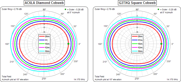
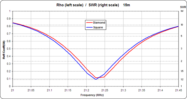
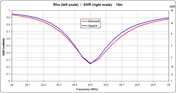
The patterns are almost identical.
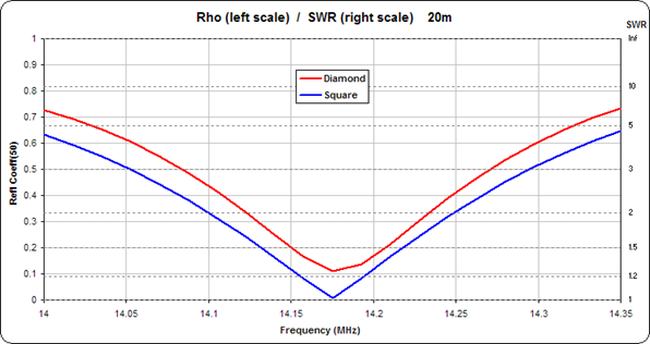
The SWR curves show a little more difference. The diamond is slightly worse on 20m, about the same on 15m, and slightly better on 10m.
Steve had a few comments on the "diamond" design:
- To keep things neat, you can run the main feedline through the spreader tube, out of the tip, and back into the balun box.
It's unlikely you would have major common mode issues on the short interconnects, but if you construct them from 4x50 ohm cables in parallel, you can produce a balanced 12.5 ohm line by connecting them: Shield1 > Shield2 > Inner3 > Inner4 and Inner1 > Inner2 > Shield3 > Shield4
Be aware that the balun box can get quite heavy, and in the diamond design it's right at the extremity of the spreader; so make sure the spreader is strong enough to take the extra weight. Alternatively just continue the 12.5 ohm line around the tip of the spreader, back through the centre of the spreader, to the balun box located and supported at the hub. And later he added this comment: I tried the "diamond configuration" with several bands today, but I confess I got tired of making up the 12.5 ohm interconnects before I'd done all five bands ... and the Rugby World Cup final on TV was proving more attractive! But I'd seen enough to be confident a 5-band version would work as predicted.Another idea I tinkered with is to combine a diamond shape with a common (aka "ganged") element feedpoint like a normal (G3TXQ or G3TPW) cobweb/CobWebb. That eliminates the need to build 12.5 ohm "interconnect" lines between separate element feedpoints as well as eliminating the need for a separate feedpoint support tube.
The outside (20m) element is in the normal cobweb shape of a square; the inner elements become more and more "squashed". Modeling shows not much difference in the patterns or SWR curves as compared to square cobweb elements.
Models:
Unzip and save to your computer then use the Open Model File button from within AutoEZ.
17/15m Coupled-Resonator Rotatable Dipoles
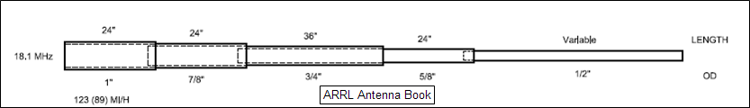
I first modeled a coupled pair of 17m/15m dipoles with stepped diameter aluminum elements. The ARRL Antenna Book gives heavy-duty and medium-duty taper schedules for 20/17/15/12/10m Yagis. I used the 17m heavy-duty one.
To keep the model simple I used the same schedule for both the 17m and 15m elements. To allow adjustments to the dimensions I used variables to control the element tip coordinates, the spacing between the elements, and the height of the 17m (upper) element.
Creating even a simple dipole with stepped diameter wires can be challenging and error-prone. AutoEZ has a tool to automate the process. Here's what the dialog window looks like to create the 15m (lower) element.
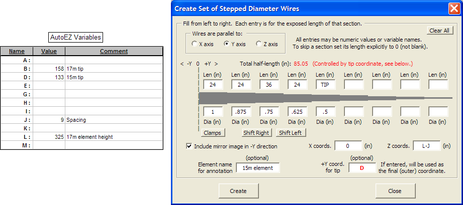
Note that the lengths and diameters of the inner sections match the ARRL taper schedule. The overall half-length is set via variable D and the height is set via a combination of L and J. The initial values for B, D, and J are just estimates. (For the element lengths K9AY suggests 477/Freq (in feet) rather than the normal 468/Freq.) Clicking "Create" generates all the appropriate End 1 and End 2 XYZ coordinates for all the wires that make up the element. In the screen grab below everyplace you see "316.000" is actually an Excel formula "=L-J" and "±133.000" is formula "=D" or "=-D".
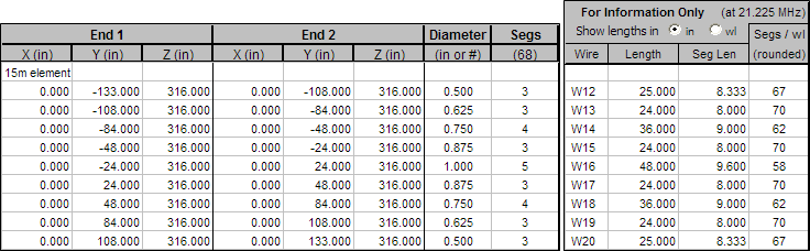
After both elements were created I let the optimizer adjust all the variables except height to get the best SWR at both 18.118 and 21.225 MHz.
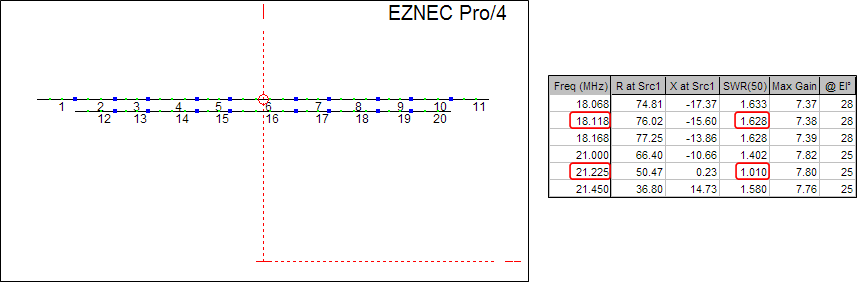
Notice that the best that could be done at 18.118 MHz is SWR ~1.6. That's because the minimum SWR of the driven dipole (the one with the transmission line connected to the center) depends mostly on the height above ground. Also note that this is one of those cases where the length for minimum SWR is not the same as the length for resonance. If the 17m element had been adjusted for resonance (jX=0) at 18.118 MHz the SWR would be 1.79 instead of 1.63.
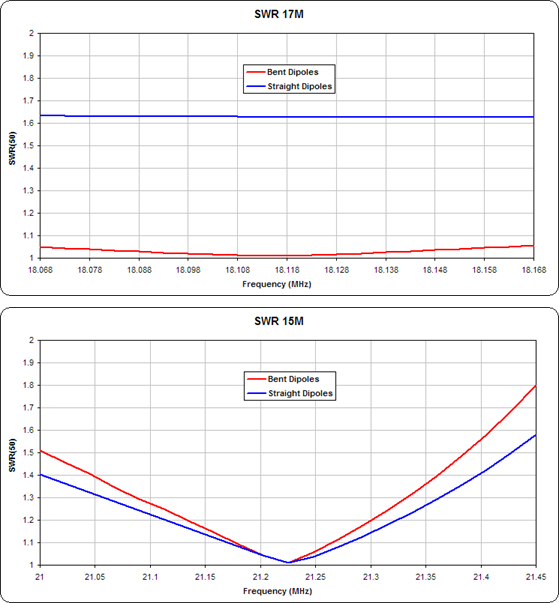
So what can be done to get a better match on 17m? If a half-wave dipole is bent into different shapes the resistance component of the feedpoint impedance at resonance changes. Here are some comparisons for a resonant 17m dipole at a height of 325 inches (1/2 wl) over average ground. All wires are 0.5" aluminum. In each case the total element length is ~1/2 wl.
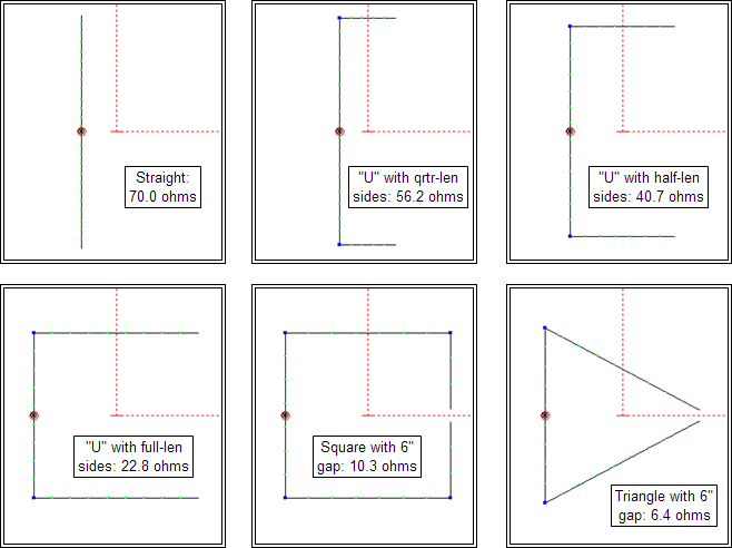
If you make the 17m (driven) element a "U" shape with somewhere between quarter-length and half-length sides, the resistance at resonance will be about 50 ohms. And you can adjust the resistance of the 15m (coupled) element to be 50 ohms by changing the spacing between the elements. For both you can adjust the tip lengths to achieve resonance.
So I modified both elements to have a "U" shape. Then once again I let the optimizer sort it all out. Here are the results.
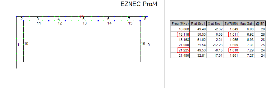
Almost a perfect match on both bands.
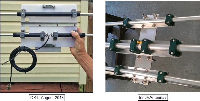
As for the physical build, a 10m/6m coupled dipole antenna was mentioned briefly on pg 94 of the August 2015 QST. The picture from that article is shown below. In that version the driven element is on the bottom; in the above models the driven element is on the top. Also shown is the professional version center assembly from Force 12/InnoVAntennas with the driven element in the middle.
Models:
Unzip and save to your computer then use the Open Model File button from within AutoEZ.
Steerable V-Beam
This simple model is intended to mimic one position of the "switchable direction" V-beam described in “A Four Wire Steerable V Beam for 10 through 40 meters” by Sam Moore, NX5Z, in the March 2011 QST. There is nothing particularly complex about the model but by looking at the Wires tab you can see how to start with a single wire and then use cascaded Rotate and Move/Copy operations, each with a variable rather than a fixed numeric value controlling the modification, to end up with a set of wires that would otherwise require some trigonometric head-scratching.
With the dimensions set as
106 ft leg lengthhere is an animation of the azimuth patterns at 20° elevation for 40m through 10m. Frequency is shown in the lower-right corner in each frame of the animation.
45 degree included angle between legs
40 ft apex height
10 ft outer ends height
The model also has an option to include a length of parallel-conductor transmission line along with a 4:1 balun at the station end of the line so you can see what impedance your tuner would have to handle on various bands.
Save to your computer then use the Open Model File button from within AutoEZ.
V-Beams are also discussed in Chapter 13 of recent editions of The ARRL Antenna Book. The CD that is bundled with the book has three sample V-Beam models in .ez format.
Self-Phasing Turnstiles
One common way to construct a turnstile antenna is with two horizontal, resonant dipoles oriented at right angles to each other. The feedpoint of one dipole is connected to the feedpoint of the second dipole via a 90° phasing line. If the characteristic impedance of the phasing line is the same as the feedpoint impedance of each independent dipole (typically ~70 ohms), the result will be currents in each dipole of equal magnitude and 90° phase difference. That will produce a horizontally polarized and (very nearly) omnidirectional pattern. The combined impedance of the connected pair will be half that of each independent dipole, typically ~35+j0 ohms.
However, the elements need not be dipoles. And by changing the geometry of the elements it is possible to a) do away with the phasing line and b) make the combined impedance of the connected pair equal to 50+j0 ohms.
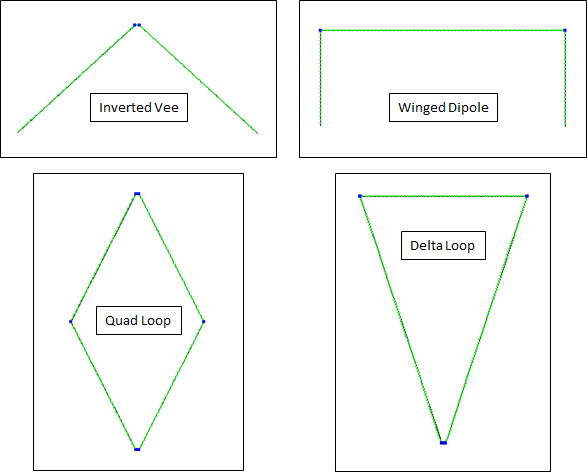
If one element of the pair is adjusted to have an independent feedpoint impedance of 50+j50 ohms while the other element has an impedance of
50-j50 ohms, when the two are connected together without a phasing line the pair will again have currents in each element of equal magnitude and 90° phase difference. But now the impedance of the connected pair will be 50+j0, convenient for direct connection to a typical amateur transmission line.The easiest way to get feedpoint impedances of 50+j50 and
50-j50 ohms is to use elements that have two "degrees of freedom" that can be adjusted separately, such as an inverted vee where the leg length and the included angle are independent. Other possibilities are "winged" dipoles (adjust totaltip-to-tip length and wing length), quad loops (adjust height and width), and delta loops (again height and width). The illustrations below show the approximate shapes needed to obtain 50±j50 feedpoint impedance values, with a slight difference needed for the +j50 vs-j50 versions. Separate images not to scale.
Models for each of the above configurations have been created in which all dimensions are controlled via variables. That, along with a little trick involving the optimizer, makes it simple to adjust each element to have an independent feedpoint impedances of either 50+j50 or
50-j50 ohms. For example, here are the variables for the quad loop model.
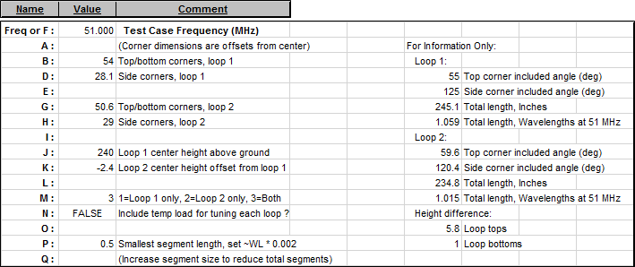
Variables B and D control the corners of loop 1 in relation to its center. Variables G and H do the same for loop 2. Variable M controls which loop is active and N places a temporary load of either
-j50 ohms (for loop 1) or +j50 ohms (for loop 2) in series with the loop feedpoint. More on that in a moment.To make loop 1 have a feedpoint impedance of 50+j50 set
M = 1 ,N = True , click the Optimizer Setup button and select variables B and D. On the Optimize tab make sure the frequency is correct and set the targets like this.
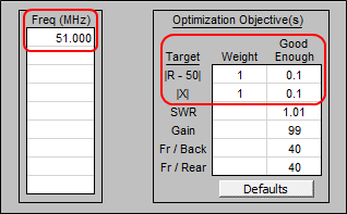
The optimizer will adjust B and D such that the loop feedpoint impedance is 50+j0 ohms (with a tolerance of 0.1 ohms for both R and jX). Then when the temporary load of
-j50 ohms is removed, the feedpoint impedance will become 50+j50 ohms.Repeat the process for loop 2. That is, set
M = 2 and optimize on G and H. This time the temporary load will be +j50 ohms and when that load is removed the optimized loop 2 feedpoint impedance of 50+j0 will become50-j50 ohms.When finished tuning both loops set
N = False . That will disable use of the temporary tuning load. Then on the Calculate tab you can run a series of test cases to verify the turnstile operation.
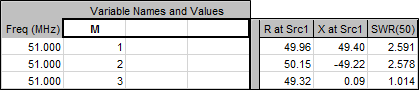
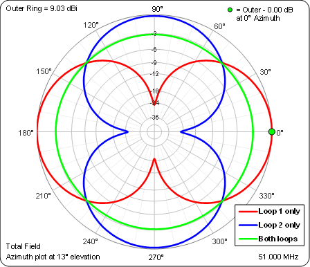
The azimuth patterns should look like this, almost perfectly omnidirectional when both loops are active.
It is also possible to create a similar "self-phasing" turnstile using just straight dipole elements that have only one "degree of freedom" (the dipole length). That is done by adding a second degree of freedom in the form of balanced loads on either side of each dipole's center feedpoint. Here is an exploded view of the center sections of such a turnstile.
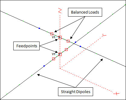
Note that for modeling purposes the two elements are physically separated by a small amount. They are then connected electrically to the common point V1 by essentially "zero" length transmission lines. (Think of the two "V1" annotations as being combined into one and located midway vertically between the two feedpoints.) Connecting the elements this way results in more accurate modeling results as opposed to connecting the elements via a separate short wire. Of course in actual construction each element would have a break in the center and both elements would be in the same plane.
The tuning procedure is even simpler. In essence, a single dipole is adjusted to have a feedpoint resistance of 50 ohms. That will typically result in the feedpoint reactance being less than (more negative than)
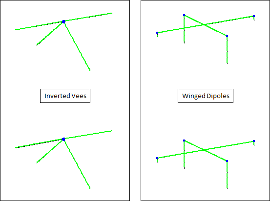
-50 jX ohms. Once that reactance value is known, balanced inductive loads (coils) will be automatically calculated and added such that one dipole's impedance is raised to 50+j50 ohms (larger inductance coils) while the other dipole's impedance is raised to only50-j50 ohms (smaller inductance coils).Not matter what type of geometry is used you can create a vertical stack of two turnstiles (two pairs of two elements), just as with stacking Yagi antennas. Because of the mutual coupling between the pairs the element shapes will be different. Here are the approximate shapes needed for a stack of inverted vee turnstiles and a stack of winged dipole turnstiles. Notice that one vee is almost a straight dipole and one winged dipole has only minimal wings.
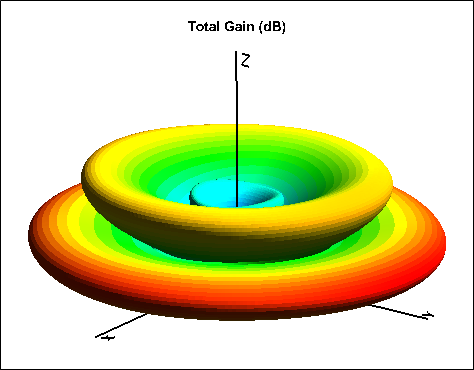
Stacking will typically increase the gain and lower the elevation angle of the main lobe as well as reduce the overhead gain. For a stack of inverted vee turnstiles at heights of 1 λ and 1.5 λ here is what the 3D pattern looks like.
Models:
The zip file below contains these AutoEZ format (*.weq) models:
Turnstiles.zip
- Self-Phasing Turnstile Inverted Vees.weq
- Self-Phasing Turnstile Winged Dipoles.weq
- Self-Phasing Turnstile Quad Loops.weq
- Self-Phasing Turnstile Delta Loops.weq
- Self-Phasing Turnstile Loaded Dipoles.weq
- Self-Phasing Stacked Turnstiles Inverted Vees.weq
- Self-Phasing Stacked Turnstiles Winged Dipoles.weq
Unzip and save to your computer then use the Open Model File button from within AutoEZ. Step-by-step instructions for tuning each model at a different frequency or for a different band are shown on the Variables tab. Also see the notes on the Wires tab concerning wire diameters and insulation properties.
References:
- Kraus, Antennas 2nd edition, 1988, section 16-7: "Turnstile Antenna" (link)
- W1VT, "A Simple 10-Meter Satellite Turnstile Antenna", QEX, November 2001
- W4RNL, "Some Notes on Turnstile Antenna Properties", QEX, March 2002
- W4RNL, "A 6-Meter Quad-Turnstile", QST, May 2002
- N3XE, "6 Meter Quad Turnstile Antenna", June 2016 (link) (home page)
In the construction articles just ignore mention of the phasing line.