Examples of using AutoEZ have been created from time to time to address questions raised on various forums and reflectors. This is a collection of such examples, in some cases slightly edited. Step by step instructions are omitted to maintain brevity.
40-30-20 Dipole Fed With Ladder Line
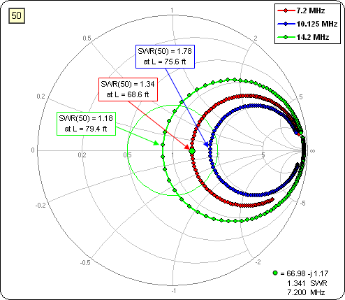
W5DXP has a nice page describing his No-Tuner All-HF-Band antenna, a 130 ft dipole used on 80m through 10m, fed in the center with varying lengths of ladder line. Here's how to see the effect of different feedline lengths for a shortened 60 ft version on the 40/30/20m bands.Define a simple dipole 60 ft long and 40 ft high (not shown), put the source at V1, and add a transmission line between the source (V1) and the feedpoint (Wire 1 / 50%) with length "=L" ft.
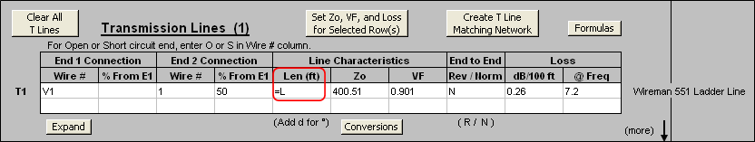
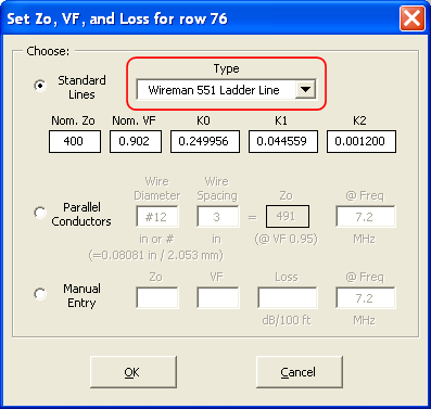
Use the Set Zo, VF, and Loss button to fill the remainder of the fields. Wireman 551 is used for this example.
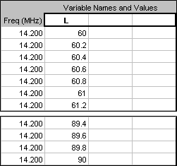
Then create a series of test cases with L ranging from 60 ft to 90 ft, all at a constant frequency. Calculate.
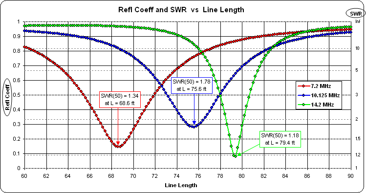
Doing the same thing for two other frequencies and capturing the traces after each set of calculations yields this rectangular chart (reflection coefficient left scale, SWR right scale) on the Custom tab.
Or this Smith chart (trace clockwise rotation = increasing line length).
Segment Lengths, AutoSeg, and Average Gain Test
K1STO discussed a spider beam antenna in the July 2005 QST. You can download the EZNEC model file from the QST Binaries page; look for the "0705ProdRev.zip" link.
Using that model merely as an example, and not because there is anything "wrong" with it, here's how to make use of the "For Information Only" columns and the "AutoSeg" dialog on the Wires tab to quickly change segmentation levels. As a result the Average Gain Test results will improve slightly.
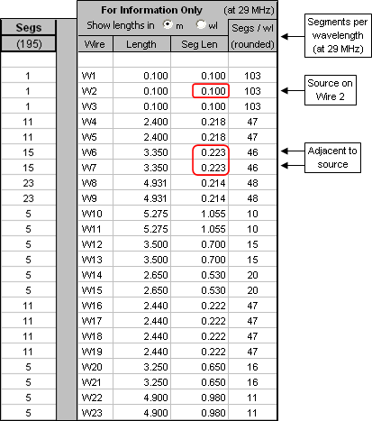
In model 'spiderbeam_3band_201510.ez' the segments on either side of the source are not the same length as the source segment. Besides that, at higher frequencies you'll get EZNEC segmentation warnings for some of the other wires since the segmentation density is less than 20 per wavelength. This is what the original segmentation looks like at 29 MHz:
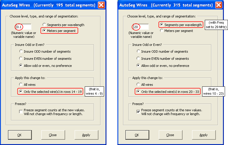
To improve the first issue set the segment length for wires 6 and 7 to (as close as possible) 0.1 m, the same as the short center segment for each of the driven elements. While you're at it, use the same segment length for wires 4-5 and 8-9. That keeps the segment boundaries on those nearby wires close to alignment which is another way to improve AGT (left image below).
To eliminate the EZNEC segmentation warnings first set the "Freq" (cell C11 on the Variables tab) to 29 MHz, then set the segmentation density for all the other wires to at least 20 segs/WL at the highest frequency of interest, assumed to be 29 MHz in this case (right image below).
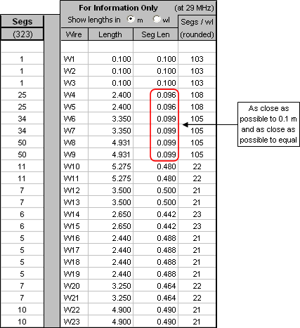
With those changes the segmentation now looks like this:
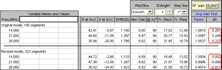
Here's a comparison of the before and after AGT results (Ground Type = Free Space):
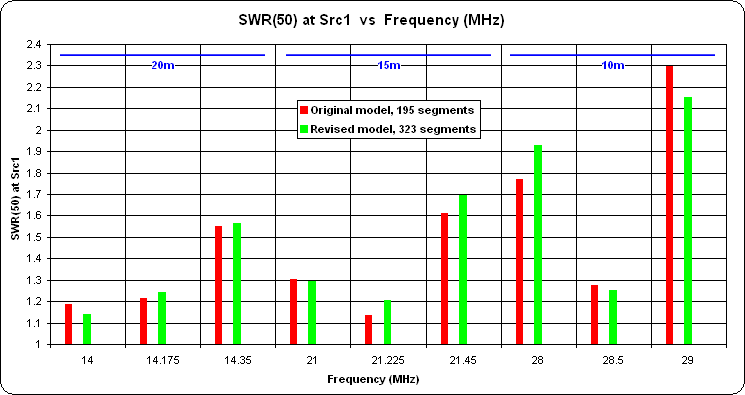
And here's a comparison of the before and after SWR values at three frequencies in each band:
Two-Element Yagi with Equal Length Elements
What? Doesn't a two-element Yagi have two different length elements, either a reflector and a driven element or a driven element and a director? Not necessarily.
The ARRL Antenna Book 10th edition (1964, cover price $2.00) has a sub-section on "Self-Resonant Parasitic Elements" for a two-element Yagi, found in Chapter 4 (Multielement Directive Arrays), section "Parasitic Arrays", sub-section "The Two-Element Beam". KL7AJ mentioned this "Yagi with Self-Resonant Elements" in a forum posting and it gave me an excuse to dig out my earliest Antenna Book from when I initially became interested in amateur radio.
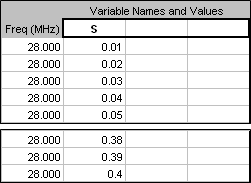
First I created a dipole element in free space having length L, with XYZ coordinates specified in wavelengths rather than feet or meters, and used the Resonate button to set the length to resonance at 28 MHz. Then I duplicated that element with a spacing between the two of S wavelengths. Hence both elements are the same length and both are self-resonant when stand-alone. Then I ran a variable sweep with S ranging from 0.01λ to 0.4λ.
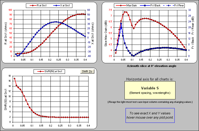
Here's the Triple sheet tab which shows several different parameters at a glance. The dip in the gain curve at spacing 0.11λ is where the parasitic (non-driven) element changes from being a director to being a reflector; that is, where the main lobe azimuth angle changes from 0° to 180°. Remember, the length of the parasitic element has not changed, only the spacing.
And here's an animation of the free space azimuth patterns. The value of S for each frame of the animation is shown in the lower right corner. The outer ring is frozen at 7.33 dBi, the gain at a spacing of 0.06λ, to allow comparison of relative strength as well as pattern shape.
As the author of this Antenna Book section said way back in 1964: "The special case of the self-resonant parasitic element is of interest, since it gives a good idea of the performance as a whole of two-element systems, even though the results can be modified by detuning [changing the length of] the parasitic element. ... If front-to-back ratio is not an important consideration, a spacing as great as 0.25 wavelength can be used without much reduction in gain, while the radiation resistance approaches that of a half-wave antenna alone."
Here's the model used for this exercise.
Dual-Band Vertical with "Autopilot" Matching Network
Here's a little modeling study which uses both the EZNEC "L Networks" feature and the AutoEZ optimizer in sort of a unique way.
In 1977 Wes Hayward, W7ZOI, described an interesting dual-band matching network. His Hints and Kinks QST submission is reproduced below.
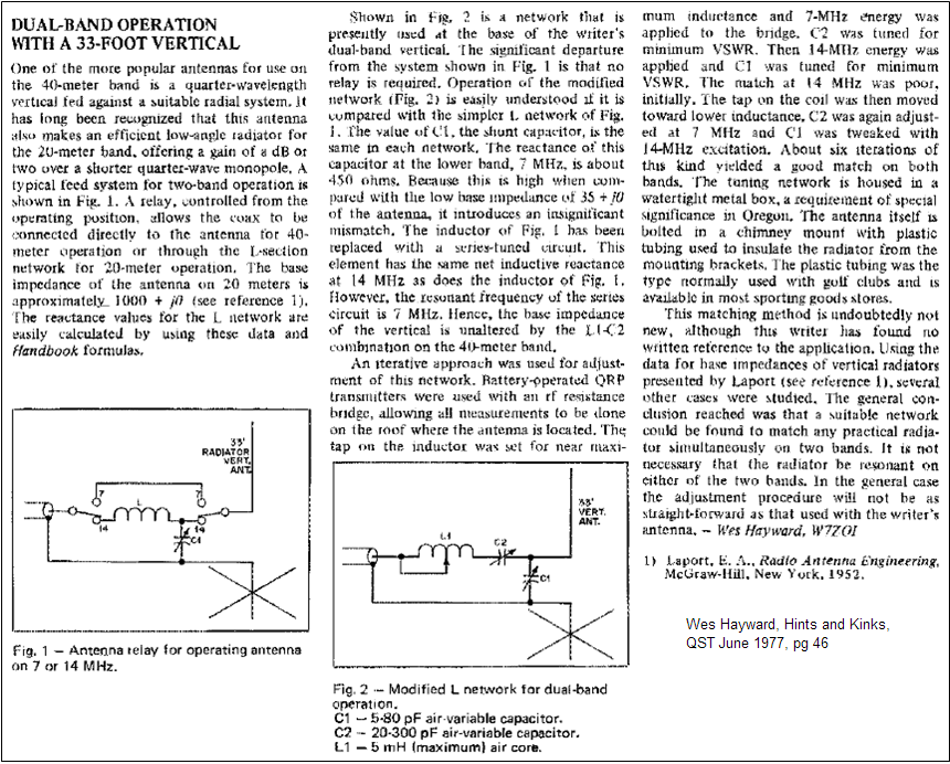
Then in 2005 Dan Richardson, K6MHE, wrote a QST article titled A 20 and 40 Meter Vertical on 'Autopilot'. And in 2008 Ryan Christman, AB8XX, did a blog entry with a corresponding YouTube video for a similar 80m/40m antenna. For those who might be interested in doing something similar, it's possible to model the entire system, antenna plus "autopilot" matching network, with EZNEC or with the AutoEZ/EZNEC combination. (Please look over at least the K6MHE article before continuing.)
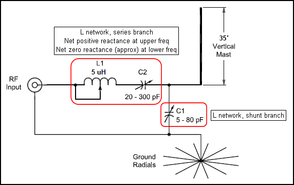
A conventional low pass L network has an inductor in the series branch and a capacitor in the shunt branch. However, EZNEC L networks can have compound components in each branch. Hence the matching network can be pictured like this (from the K6MHE article Fig 2).
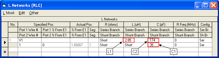
Here is the AutoEZ L Networks table with variables K-L-M being used for the component C1-L1-C2 values. The source is on V1, the network input port. The network output port is the antenna feedpoint.

The following extract from the AutoEZ Variables sheet tab shows the initial values for the K6MHE 40m/20m setup. Instructions for setting the initial network component values (variables K-L-M) are found in additional comments on the sheet, not shown. (The scratchpad area of the sheet has the necessary Excel formulas for computing the initial K-L values for an impedance match at the upper frequency and the initial M value for a net zero reactance at the lower frequency.)
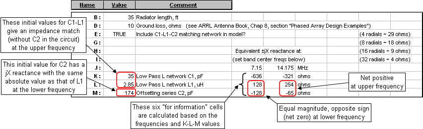
Note that ground loss due to a less than perfect radial field is simulated using variable D in conjunction with MININEC-type ground; actual radials are not included in the model (although you may add them if you wish and change to High Accuracy ground).
With the C1-L1-C2 component values as set above, the L network looks like this when the model is passed to EZNEC.
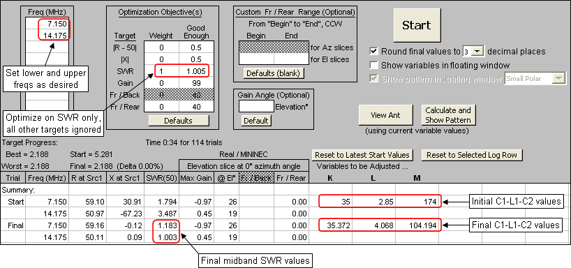
Once the initial network values are set, the AutoEZ optimizer can be used to adjust components C1-L1-C2 (variables K-L-M) to produce the lowest possible SWR at the two midband frequencies.
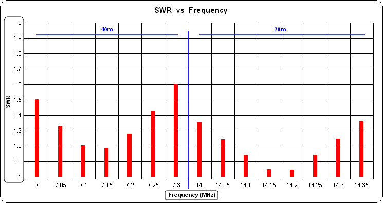
After optimization, here are the final SWR values for seven 40m frequencies and eight 20m frequencies. This is similar to Fig 5 in the K6MHE article except that all frequencies are shown on a single chart. (Blue markup added for clarity.)
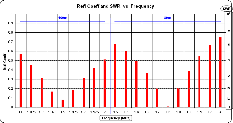
Doing the same kind of analysis for 160m/80m (with radiator length B = 132 ft, although not many folks have a full-size vertical for 160) gives these SWR values, this time shown with a different scale for SWR (on the right). The midband SWR values are fine (remember, right scale) but because of the relatively larger widths of 160 and 80 the band edge SWR values are higher.
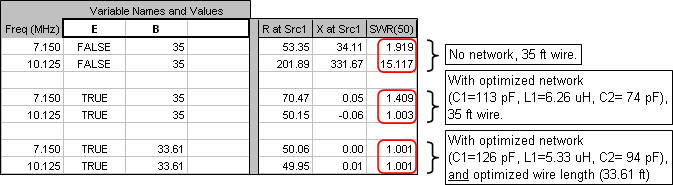
The examples above were for 40/20 and 160/80 but the two bands need not be harmonically related. Here is an example for 40/30 with three scenarios: First was a 35 ft vertical at 7.15 and 10.125 MHz with no matching network. Second was adding a "dual-band autopilot" L network with optimized component values. And third was allowing the optimizer to vary the wire length as well as the network values; that is, optimizing on 4 variables instead of 3 variables. In all cases the model had 10 ohms of assumed ground loss.
Here is the model used for this study.
Download that file, use the Open Model File button, then tab to the Variables sheet and read the comments to get started. As downloaded, the model is ready to be optimized (Optimize tab, Start button) and then calculated over multiple frequencies (Calculate tab, Calculate All button).
Of course, results are only as good as the model. If you have an analyzer and can measure the actual unmatched feedpoint impedance (R±jX) at your chosen target frequency in each band, you can then adjust variables B and D (with E = False, no network) to make the calculated R and X match the measured R and X. Then model the matching network.
Ground Mounted Vertical, Resonant Height vs Element Diameter
If a "shortening factor" is defined as the ratio between the height of a resonant ground mounted vertical and a free space quarter wavelength, the following curves show the factors for element diameters ranging from 0.125" (~ #8 AWG) to 4" at both 3.75 MHz and 28.5 MHz.
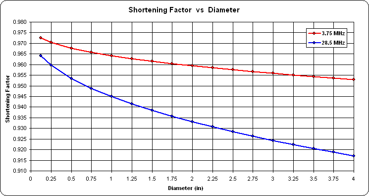
For 3.75 MHz the factors vary from 0.973 to 0.953; for 28.5 MHz, from 0.964 to 0.917. Note that the 28.5 MHz factors do not correspond to Table 1 in the Antenna Compendium Volume 2 article by Doty et al. The Doty ACV2 measurements were done with the vertical element mounted over an elevated counterpoise, not ground mounted.
Calculations for the above chart are easy using the Resonate button of AutoEZ. The procedure is shown here.
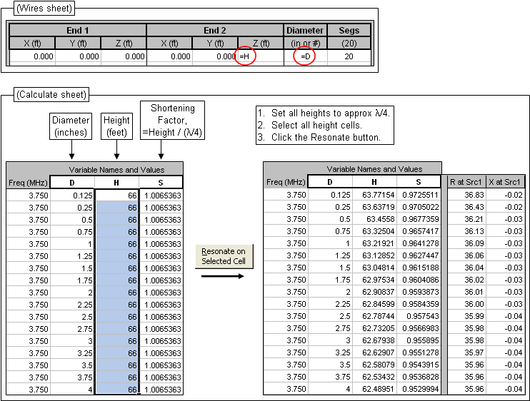
If you'd like to duplicate these results, or run calculations for other frequencies, the following model file is suitable for use with the free demo version of AutoEZ in conjunction with any version of EZNEC v. 5.0.60 or newer including the EZNEC Pro+ v. 7.0 program which is now free.
Download that file, use the AutoEZ Open Model File button, tab to the Calculate sheet, select all the H values (cells D11-D27), and click the Resonate button. Or change all the frequencies to your new choice and set all the H values to approximately λ/4 at that frequency (initial value not critical), then select all the H values and click the Resonate button.
To produce a plot of the results, tab to the Custom sheet and choose "Variable 3" (Shortening Factor) for the Y axis and "Variable 1" (Diameter) for the X axis.
Modeling 8-Circle Arrays
Concerning 8-circle receiving arrays, I was curious about the relationship between array size, element phasing, and number of active elements so I created models where the array diameter and phasing can be controlled via variables. For example, here's the AutoEZ Variables sheet tab for a "W8JI type" (aka BroadSide/End-Fire or BSEF, 4 elements in use) 8-circle array.

Since everything is controlled by variables you can run "variable sweeps" changing one or more parameters. Here's the W8JI array with the spacing (B) held constant while the phase delay (P) is swept from 80 to 140 degrees. For each test case AutoEZ will automatically calculate the RDF (last column).

When the calculations finish you can step through the 2D patterns. Here are the elevation and azimuth (at 20° TOA) patterns for 0.604 wl broadside spacing and 125° phasing, as shown by B and P in the lower right corner.

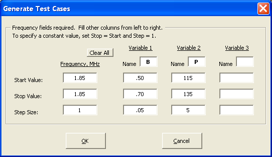
You can run similar sweeps changing the array size while holding the phase delay constant, or hold both size and phase constant and do a frequency sweep, or use the "Generate Test Cases" button to create any combination. For example, the setup below would vary broadside spacing B from 0.50 to 0.70 wavelengths; for each B the phase delay P would be varied from 115 to 135 degrees; all at a constant frequency of 1.85 MHz.
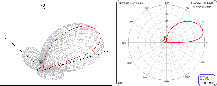
The model for a "Hi-Z type" (8 elements in use) 8-circle array is similar except that array size is specified in feet (or meters) rather than wavelengths. Here's the 3D pattern for a Hi-Z array with diameter 200 ft and ±106° phasing, along with the 2D elevation pattern.
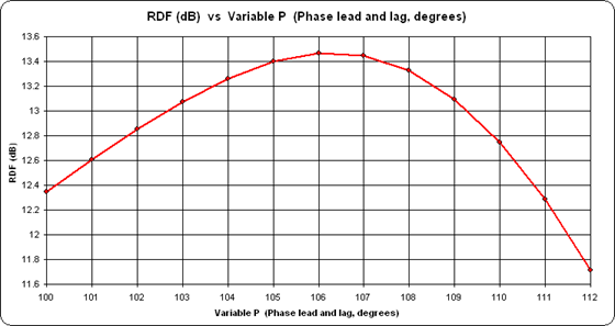
And here's how the RDF for a 200 ft Hi-Z array varies as the phase is swept from ±100° to ±112°.
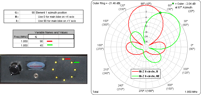
The models also have a variable to control the azimuth direction of the main lobe. That lets you change the direction just by changing (or doing a sweep on) a single variable. So you can easily: 1) see how the azimuth patterns overlap as the array is steered in 45° steps, and 2) compare patterns against other models which may be fixed in a particular direction.
For case 1, here's how the Hi-Z type array patterns would overlap as you turn the knob on the control box. This is for a 200 ft diameter array with ±106° phasing, 20° TOA for the patterns. Compass rose angles are shown in parenthesis on the polar chart.
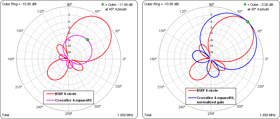
For case 2, this is how the W8JI type array with 0.604 wl broadside spacing and 125° phasing compares against a 4-square receiving array with 0.125 wl element spacing and Crossfire feeding. Both arrays use the same basic element, the top hat model RXvrhat.ez from the W8JI Small Vertical Arrays page.
At a 20° TOA the 4-square has a gain of -22.43 dBi compared to -10.95 dBi for the 8-circle. (But the RDF is only about 1 dB lower for a diameter of 94 ft compared to 348 ft for the 8-circle.) In order to get an accurate comparison of the pattern shapes on the same polar chart, the gain of the 4-square has been normalized to that of the 8-circle by reducing the value of the swamping resistors. Original gain below on left, normalized gain below on right.
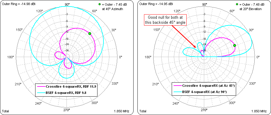
The 4-square can be fed either as Crossfire or BroadSide/End-Fire using exactly the same phasing lines, a neat idea picked up from IV3PRK. In the patterns below, the swamping resistors are back at the normal values (to give 75+j0 at the feedpoint for a standalone element). With Crossfire feeding the gain at 20° TOA is down 7.45 dB compared to BSEF feeding but the RDF is 2.1 dB better, below left. Note that a design criteria for IV3PRK was good rejection at backside 45° elevation, below right.
For both of the array types, I created one model using W8JI-style top hat loaded vertical elements and a second model using simple aluminum tube elements per the four-section, 23.25 ft, Hi-Z AL-24 antenna. Here are the models.
W8JI_8_Circle__TopHat.weq
W8JI_8_Circle__AL-24.weq
Hi-Z_8_Circle__TopHat.weq
Hi-Z_8_Circle__AL-24.weqIn all the models, a single variable (X) controls the segmentation. You can reduce that to speed up the calculations. You can also run a sweep on X to do a convergence test for model accuracy.
Here's the 4-squareRX model with a variable that switches between Crossfire feed and BSEF feed.
For comparison with the above arrays, here's the W8WWV "Benchmark Beverage" model. With this one you can "sweep" the length and/or other parameters.
References:
ON4UN's Low-Band DXing by John Devoldere, Chapters 7 and 11:
https://www.arrl.org/shop/ON4UN-s-Low-Band-DXing
For "W8JI type" arrays:
http://w8ji.com/small_vertical_arrays.htm
http://n3ujj.com/manuals/8%20Circle%20Vertical%20Array%20for%20Low%20Band%20Receiving.pdf
http://www.dxengineering.com/parts/dxe-rca8b-sys-3p
http://static.dxengineering.com/global/images/instructions/dxe-rca8b-sys-3p-rev3.pdfFor "Hi-Z type" arrays:
http://www.k7tjr.com/need.htm
http://www.kkn.net/dayton2014/HiZ_DAYTON_2014_7n2.pdf
http://www.hizantennas.com/HiZ8-160&80_users_guide.pdf
http://www.hizantennas.com/Hiz_8_160&80_manual.pdf
http://www.dxengineering.com/parts/hiz-8a-lv2-160-2For the IV3PRK dual-feed 4-square (follow the links on the left side of the page):
http://www.iv3prk.it/rx-antennas.htm
For the W8WWV Beverage:
http://www.seed-solutions.com/gregordy/Amateur%20Radio/Experimentation/Beverage.htm
2014 Contest Univesity presentation by W3LPL on Receiving Antennas:
http://www.contestuniversity.com/attachments/W3LPL_Receiving_Antennas_2014.pptx